Harry Markowitz and the Birth of Portfolio Theory

Most of the ideas in Chapter 7 date back to an article written in 1952 by Harry Markowitz.^[1] Markowitz drew attention to the common practice of portfolio diversification and showed exactly how an investor can reduce the standard deviation of portfolio returns by choosing stocks that do not move exactly together. But Markowitz did not stop there; he went on to work out the basic principles of portfolio construction. These principles are the foundation for much of what has been written about the relationship between risk and return.

We begin with Figure 8.1, which shows a histogram of the daily returns on IBM stock from 1997 to 2017. On this histogram we have superimposed a bell-shaped normal distribution.

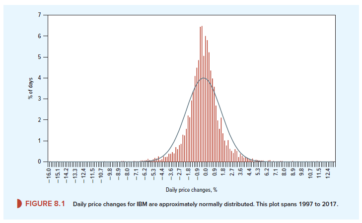
The result is typical: When measured over a short interval, the past rates of return on any stock conform fairly closely to a normal distribution.

Normal distributions can be completely defined by two numbers. One is the average or expected value; the other is the variance or standard deviation. Now you can see why we discussed the calculation of expected return and standard deviation in Chapter 7. They are not just arbitrary measures: If returns are normally distributed, expected return and standard deviation are the only two measures that an investor need consider.

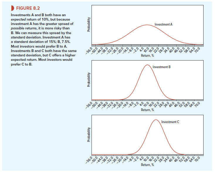
Figure 8.2 pictures the distribution of possible returns from three investments. Investments A and B offer an expected return of 10%, but A has the much wider spread of possible out­comes. Its standard deviation is 15%; the standard deviation of B is 7.5%. Most investors dis­like uncertainty and would therefore prefer B to A.

Now compare investments B and C. This time both have the same standard deviation, but the expected return is 20% from stock C and only 10% from stock B. Most investors like high expected return and would therefore prefer C to B.

1. Combining Stocks into Portfolios

Think back to Section 7-3, where you were wondering whether to invest 60% of your savings in the shares of Southwest Airlines and 40% in those of Amazon. You decided that South­west Airlines offered an expected return of 15.0% and Amazon offered an expected return of 10.0%. After looking back at the past variability of the two stocks, you also decided that the standard deviation of returns was 27.9% for Southwest and 26.6% for Amazon.

The expected return on this portfolio is 13%, simply a weighted average of the expected returns on the two holdings. What about the risk of such a portfolio? We know that thanks to diversifica­tion the portfolio risk is less than the average of the risks of the separate stocks. In fact, on the basis of past experience the standard deviation of this portfolio is 22.0%, well below that of either stock.

The curved blue line in Figure 8.3 shows the expected return and risk that you could achieve by different combinations of the two stocks. Which of these combinations is best depends on your stomach. If you want to stake all on getting rich quickly, you should put all your money in Southwest Airlines. If you want a more peaceful life, you should split your money between the two stocks.

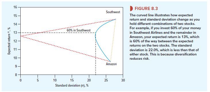
We saw in Chapter 7 that the gain from diversification depends on how highly the stocks are correlated. Fortunately, on past experience, there is only a modest correlation between the returns of Southwest Airlines and Amazon (p = +.26). If their stocks moved in exact lockstep (p = +1), there would be no gains at all from diversification. You can see this by the gold dotted line in Figure 8.3. The red dotted line in the figure shows a second extreme (and equally unrealistic) case in which the returns on the two stocks are perfectly negatively correlated (p = -1). If this were so, there is a combination of the two stocks that would have no risk.

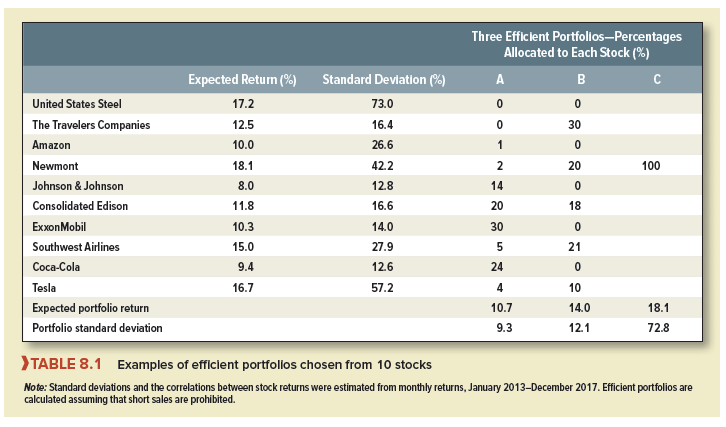
In practice, you are not limited to investing in just two stocks. For example, you could decide to choose a portfolio from the 10 stocks listed in the first column of Table 8.1. After analyzing the prospects for each firm and talking to your stockbroker, you come up with fore­casts of their returns. You are most optimistic about the outlook for Newmont and forecast that it will provide a return of 18.1%. At the other extreme, you predict a return of only 8% for Johnson & Johnson. You use data for the past five years to estimate the risk of each stock and the correlation between the returns on each pair of stocks.^[6]

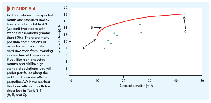
Now look at Figure 8.4. Each dot marks the combination of risk and return offered by a different individual security.

By holding different proportions of the 10 securities, you can obtain an even wider selec­tion of risk and return, but which combination is best? Well, what is your goal? Which direction do you want to go? The answer should be obvious: You want to go up (to increase expected return) and to the left (to reduce risk). Go as far as you can, and you will end up with one of the portfolios that lies along the red line. Markowitz called them efficient portfolios. They offer the highest expected return for any level of risk.

We will not calculate the entire set of efficient portfolios here, but you may be inter­ested in how to do it. Think back to the capital rationing problem in Section 5-4. There we wanted to deploy a limited amount of capital investment in a mixture of projects to give the highest NPV. Here we want to deploy an investor’s funds to give the highest expected return for a given standard deviation. In principle, both problems can be solved by hunt­ing and pecking—but only in principle. To solve the capital rationing problem, we can employ linear programming; to solve the portfolio problem, we would turn to a variant of linear programming known as quadratic programming. Given the expected return and standard deviation for each stock, as well as the correlation between each pair of stocks, we could use a standard quadratic computer program to search out the set of efficient portfolios.

Three of these efficient portfolios are marked in Figure 8.4. Their compositions are summarized in Table 8.1. Portfolio C offers the highest expected return: It is invested entirely in one stock, Newmont. Portfolio A offers the minimum risk; you can see from Table 8.1 that it has large holdings in ExxonMobil, Consolidated Edison, Coca-Cola, and Johnson & Johnson, which have the lowest standard deviations. However, the portfolio also has a small holding in Tesla even though it is individually risky. The reason? On past evi­dence, Tesla’s fortunes are almost uncorrelated with those of other stocks and so provide additional diversification.

Table 8.1 also shows the composition of a third efficient portfolio with intermediate levels of risk and expected return.

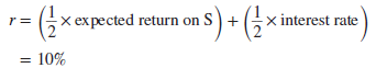
Of course, large investment funds can choose from thousands of stocks and thereby achieve a wider choice of risk and return. This choice is represented in Figure 8.5 by the shaded, broken-egg-shaped area. The set of efficient portfolios is again marked by the red curved line.

2. We Introduce Borrowing and Lending

Now we introduce yet another possibility. Suppose that you can also lend or borrow money at some risk-free rate of interest rf. If you invest some of your money in Treasury bills (i.e., lend money) and place the remainder in common stock portfolio S, you can obtain any combina­tion of expected return and risk along the straight line joining rf and S in Figure 8.5. Since borrowing is merely negative lending, you can extend the range of possibilities to the right of S by borrowing funds at an interest rate of rf and investing them as well as your own money in portfolio S.

Let us put some numbers on this. Suppose that portfolio S has an expected return of 15% and a standard deviation of 16%. Treasury bills offer an interest rate (rf) of 5% and are risk­free (i.e., their standard deviation is zero). If you invest half your money in portfolio S and lend the remainder at 5%, the expected return on your investment is likewise halfway between the expected return on S and the interest rate on Treasury bills:

And the standard deviation is halfway between the standard deviation of S and the standard deviation of Treasury bills:^[7]

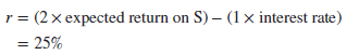
Or suppose that you decide to go for the big time: You borrow at the Treasury bill rate an amount equal to your initial wealth, and you invest everything in portfolio S. You have twice your own money invested in S, but you have to pay interest on the loan. Therefore your expected return is

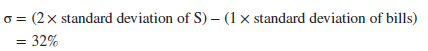
And the standard deviation of your investment is

You can see from Figure 8.5 that when you lend a portion of your money, you end up partway between rf and S; if you can borrow money at the risk-free rate, you can extend your possibili­ties beyond S. You can also see that regardless of the level of risk you choose, you can get the highest expected return by a mixture of portfolio S and borrowing or lending. S is the best efficient portfolio. There is no reason ever to hold, say, portfolio T.

If you have a graph of efficient portfolios, as in Figure 8.5, finding this best efficient port­folio is easy. Start on the vertical axis at rf, and draw the steepest line you can to the curved red line of efficient portfolios. That line will be tangent to the red line. The efficient portfolio at the tangency point is better than all the others. Notice that it offers the highest ratio of risk premium to standard deviation. This ratio of the risk premium to the standard deviation is called the Sharpe ratio:

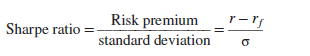
Investors track Sharpe ratios to measure the risk-adjusted performance of investment manag­ers. (Take a look at the mini-case at the end of this chapter.)

We can now separate the investor’s job into two stages. The first step is to select the best portfolio of common stocks—S in our example. The second step is to blend this portfolio with borrowing or lending to match the investor’s willingness to bear risk. Each investor, therefore, should put money into just two benchmark investments—a risky portfolio S and a risk-free loan (borrowing or lending).

What does portfolio S look like? If you have better information than your rivals, you will want the portfolio to include relatively large investments in the stocks you think are

undervalued. But in a competitive market, you are unlikely to have a monopoly of good ideas. In that case, there is no reason to hold a different portfolio of common stocks from any­body else. In other words, you might just as well hold the market portfolio. That is why many professional investors invest in a market-index portfolio and why most others hold well- diversified portfolios.

Source:  Brealey Richard A., Myers Stewart C., Allen Franklin (2020), Principles of Corporate Finance, McGraw-Hill Education; 13th edition.