The post What is Corporate Finance? Fundamentals, Principles and Features appeared first on HKT Consultant.
]]>A business undertakes such decisions to achieve pre-set financial goals while ensuring maximisation of shareholder value. Apart from understanding what corporate finance is, understand what it covers.
Corporate financeSee more from basic to advanced
















The post What is Corporate Finance? Fundamentals, Principles and Features appeared first on HKT Consultant.
]]>The post Corporate Investment and Financing Decisions appeared first on HKT Consultant.
]]>Take a corporate bond as a second example. The corporation sells the bond to investors in exchange for the promise to pay interest on the bond and to pay off the bond at its maturity. The bond is a financial asset, and also a security, because it can be held and traded by many investors in financial markets. Securities include bonds, shares of stock, and a dizzying variety of specialized instruments. We describe bonds in Chapter 3, stocks in Chapter 4, and other securities in later chapters.
This suggests the following definitions:
Investment decision = purchase of real assets
Financing decision = sale of securities and other financial assets
But these equations are too simple. The investment decision also involves managing assets already in place and deciding when to shut down and dispose of assets when they are no longer profitable. The corporation also has to manage and control the risks of its investments. The financing decision includes not just raising cash today but also meeting its obligations to banks, bondholders, and stockholders that have contributed financing in the past. For example, the corporation has to repay its debts when they become due. If it cannot do so, it ends up insolvent and bankrupt. Sooner or later the corporation will also want to pay out cash to its shareholders.[1]
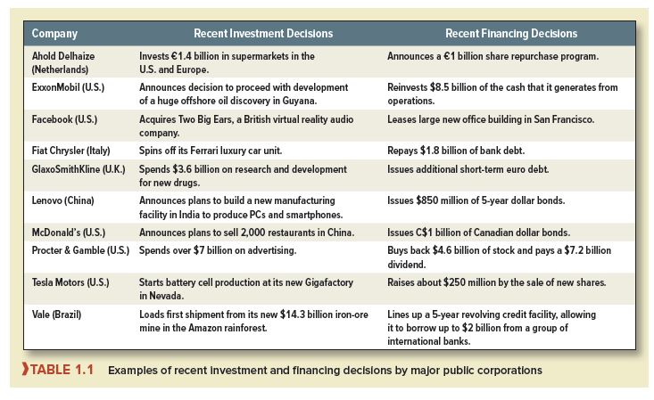
Let’s go to more specific examples. Table 1.1 lists 10 corporations from all over the world. We have chosen very large public corporations that you are probably already familiar with. You may have used Facebook to chat with your friends, eaten at McDonald’s, or used Crest toothpaste.
1. Investment Decisions
The second column of Table 1.1 shows an important recent investment decision for each corporation. These investment decisions are often referred to as capital budgeting or capital expenditure (CAPEX) decisions because most large corporations prepare an annual capital budget listing the major projects approved for investment. Some of the investments in Table 1.1, such as ExxonMobil’s new oil field or Lenovo’s factory, involve the purchase of tangible assets—assets that you can touch and kick. However, corporations also need to invest in intangible assets, such as research and development (R&D), advertising, and computer software. For example, GlaxoSmithKline and other major pharmaceutical companies invest billions every year on R&D for new drugs. Similarly, consumer goods companies such as Procter & Gamble invest huge sums in advertising and marketing their products. These outlays are investments because they build know-how, brand recognition, and reputation for the long run.
Today’s capital investments generate future cash returns. Sometimes the cash inflows last for decades. For example, many U.S. nuclear power plants, which were initially licensed by the Nuclear Regulatory Commission to operate for 40 years, are now being re-licensed for 20 more years and may be able to operate efficiently for 80 years overall.
Of course, not all investments have such distant payoffs. For example, Walmart spends about $50 billion each year to stock up its stores and warehouses before the holiday season. The company’s return on this investment comes within months as the inventory is drawn down and the goods are sold.
In addition, financial managers know (or quickly learn) that cash returns are not guaranteed. An investment could be a smashing success or a dismal failure. For example, the Iridium communications satellite system, which offered instant telephone connections worldwide, soaked up $5 billion of investment before it started operations in 1998. It needed 400,000 subscribers to break even, but attracted only a small fraction of that number. Iridium defaulted on its debt and filed for bankruptcy in 1999. The Iridium system was sold a year later for just $25 million. (Iridium has recovered and is now profitable, however.)[2]
Among the contenders for the all-time worst investment was Hewlett-Packard’s (HP) purchase of the British software company Autonomy. HP paid $11.1 billion for Autonomy. Just 13 months later, it wrote down the value of this investment by $8.8 billion. HP claimed that it was misled by improper accounting at Autonomy. Nevertheless, the acquisition was a disastrous investment, and HP’s CEO was fired in short order.
In some cases, the costs and risks of an investment can be huge. For example, the cost of developing the Gorgon natural gas field in Australia has been estimated at more than $40 billion. But do not think of the financial manager as making such large investments on a daily basis. Most investment decisions are smaller and simpler, such as the purchase of a truck, machine tool, or computer system. Corporations make thousands of these smaller investment decisions every year. The cumulative amount of small investments can be just as large as that of the occasional big investments.
Also, financial managers do not make major investment decisions in solitary confinement. They may work as part of a team of engineers and managers from manufacturing, marketing, and other business functions.
2. Financing Decisions
The third column of Table 1.1 lists a recent financing decision by each corporation. A corporation can raise money from lenders or from shareholders. If it borrows, the lenders contribute the cash, and the corporation promises to pay back the debt plus a fixed rate of interest. If the shareholders put up the cash, they do not get a fixed return, but they hold shares of stock and therefore get a fraction of future profits and cash flow. The shareholders are equity investors, who contribute equity financing. The choice between debt and equity financing is called the capital structure decision. Capital refers to the firm’s sources of long-term financing.
The financing choices available to large corporations seem almost endless. Suppose the firm decides to borrow. Should it borrow from a bank or borrow by issuing bonds that can be traded by investors? Should it borrow for 1 year or 20 years? If it borrows for 20 years, should it reserve the right to pay off the debt early? Should it borrow in Paris, receiving and promising to repay euros, or should it borrow dollars in New York?
Corporations raise equity financing in two ways. First, they can issue new shares of stock. The investors who buy the new shares put up cash in exchange for a fraction of the corporation’s future cash flow and profits. Second, the corporation can take the cash flow generated by its existing assets and reinvest that cash in new assets. In this case the corporation is reinvesting on behalf of existing stockholders. No new shares are issued.
What happens when a corporation does not reinvest all of the cash flow generated by its existing assets? It may hold the cash in reserve for future investment, or it may pay the cash back to its shareholders. Table 1.1 shows that Procter & Gamble paid back $4.6 billion to its stockholders by repurchasing shares. This was in addition to $7.2 billion paid out as cash dividends. The decision to pay dividends or repurchase shares is called the payout decision. We cover payout decisions in Chapter 16.
In some ways, financing decisions are less important than investment decisions. Financial managers say that “value comes mainly from the asset side of the balance sheet.” In fact, the most successful corporations sometimes have the simplest financing strategies. Take Microsoft as an example. It is one of the world’s most valuable corporations. In December 2017, Microsoft shares traded for about $88 each. There were 7.7 billion shares outstanding. Therefore Microsoft’s overall market value—its market capitalization or market cap—was $88 X 7.7 = $680 billion. Where did this market value come from? It came from Microsoft’s product development, from its brand name and worldwide customer base, from its research and development, and from its ability to make profitable future investments. The value did not come from sophisticated financing. Microsoft’s financing strategy is very simple: It carries no debt to speak of and finances almost all investment by retaining and reinvesting cash flow.
Financing decisions may not add much value, compared with good investment decisions, but they can destroy value if they are stupid or if they are ambushed by bad news. For example, after a consortium of investment companies bought the energy giant TXU in 2007, the company took on an additional $50 billion of debt. This may not have been a stupid decision, but it did prove nearly fatal. The consortium did not foresee the expansion of shale gas production and the resulting sharp fall in natural gas and electricity prices. In 2014, the company (renamed Energy Future Holdings) was no longer able to service its debts and filed for bankruptcy.
Business is inherently risky. The financial manager needs to identify the risks and make sure they are managed properly. For example, debt has its advantages, but too much debt can land the company in bankruptcy, as the buyers of TXU discovered. Companies can also be knocked off course by recessions, by changes in commodity prices, interest rates and exchange rates, or by adverse political developments. Some of these risks can be hedged or insured, however, as we explain in Chapters 26 and 27.
3. What Is a Corporation?
We have been referring to “corporations.” Before going too far or too fast, we need to offer some basic definitions. Details follow in later chapters.
A corporation is a legal entity. In the view of the law, it is a legal person that is owned by its shareholders. As a legal person, the corporation can make contracts, carry on a business, borrow or lend money, and sue or be sued. One corporation can make a takeover bid for another and then merge the two businesses. Corporations pay taxes—but cannot vote!
In the United States, corporations are formed under state law, based on articles of incorporation that set out the purpose of the business and how it is to be governed and operated.3 For example, the articles of incorporation specify the composition and role of the board of directors.4 A corporation’s directors are elected by the shareholders. They choose and advise top management and must sign off on important corporate actions, such as mergers and the payment of dividends to shareholders.
A corporation is owned by its shareholders but is legally distinct from them. Therefore the shareholders have limited liability, which means that they cannot be held personally responsible for the corporation’s debts. When the U.S. financial corporation Lehman Brothers failed in 2008, no one demanded that its stockholders put up more money to cover Lehman’s massive debts. Shareholders can lose their entire investment in a corporation, but no more.
When a corporation is first established, its shares may be privately held by a small group of investors, such as the company’s managers and a few backers. In this case, the shares are not publicly traded and the company is closely held. Eventually, when the firm grows and new shares are issued to raise additional capital, its shares are traded in public markets such as the New York Stock Exchange. These corporations are known as public companies. Most well-known corporations in the U.S. are public companies with widely dispersed shareholdings. In other countries, it is more common for large corporations to remain in private hands, and many public companies may be controlled by just a handful of investors. The latter category includes such well-known names as Volkswagen (Germany), Alibaba (China), Softbank (Japan), and the Swatch Group (Switzerland).
A large public corporation may have hundreds of thousands of shareholders, who own the business but cannot possibly manage or control it directly. This separation of ownership and control gives corporations permanence. Even if managers quit or are dismissed and replaced, the corporation survives. Today’s stockholders can sell all their shares to new investors without disrupting the operations of the business. Corporations can, in principle, live forever, and in practice, they may survive many human lifetimes. One of the oldest corporations is the Hudson’s Bay Company, which was formed in 1670 to profit from the fur trade between northern Canada and England. The company still operates as one of Canada’s leading retail chains.
The separation of ownership and control can also have a downside, for it can open the door for managers and directors to act in their own interests rather than in the stockholders’ interest. We return to this problem later in the chapter.
There are other disadvantages to being a corporation. One is the cost, in both time and money, of managing the corporation’s legal machinery. These costs are particularly burdensome for small businesses. There is also an important tax drawback to corporations in the United States. Because the corporation is a separate legal entity, it is taxed separately. So corporations pay tax on their profits, and shareholders are taxed again when they receive dividends from the company or sell their shares at a profit. By contrast, income generated by businesses that are not incorporated is taxed just once as personal income.
Almost all large and medium-sized businesses are corporations, but the nearby box describes how smaller businesses may be organized.
4. The Role of the Financial Manager
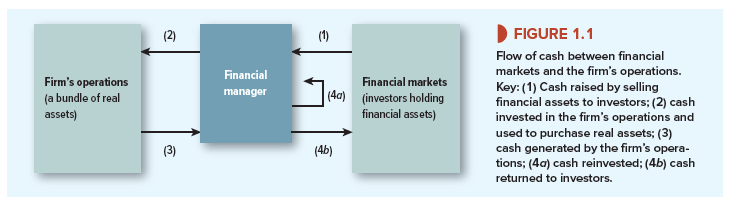
What is the essential role of the financial manager? Figure 1.1 gives one answer. The figure traces how money flows from investors to the corporation and back to investors again. The flow starts when cash is raised from investors (arrow 1 in the figure). The cash could come from banks or from securities sold to investors in financial markets. The cash is then used to pay for the real assets (capital investment projects) needed for the corporation’s business (arrow 2). Later, as the business operates, the assets produce cash inflows (arrow 3). That cash is either reinvested (arrow 4a) or returned to the investors who furnished the money in the first place (arrow 4b). Of course, the choice between arrows 4a and 4b is constrained by the promises made when cash was raised at arrow 1. For example, if the firm borrows money from a bank at arrow 1, it must repay this money plus interest at arrow 4b.
You can see examples of arrows 4a and 4b in Table 1.1. ExxonMobil financed its new projects by reinvesting earnings (arrow 4a). Procter & Gamble decided to return cash to shareholders by paying cash dividends and by buying back its stock (arrow 4b).
Notice how the financial manager stands between the firm and outside investors. On the one hand, the financial manager helps manage the firm’s operations, particularly by helping to make good investment decisions. On the other hand, the financial manager deals with investors—not just with shareholders but also with financial institutions such as banks and with financial markets such as the New York Stock Exchange.
Source: Brealey Richard A., Myers Stewart C., Allen Franklin (2020), Principles of Corporate Finance, McGraw-Hill Education; 13th edition.
The post Corporate Investment and Financing Decisions appeared first on HKT Consultant.
]]>The post The Financial Goal of the Corporation appeared first on HKT Consultant.
]]>Major corporations may have hundreds of thousands of shareholders. There is no way that these shareholders can be actively involved in management; it would be like trying to run New York City by town meetings. Authority has to be delegated to professional managers. But how can the company’s managers make decisions that satisfy all the shareholders? No two shareholders are exactly the same. Some may plan to cash in their investments next year; others may be investing for a distant old age. Some may be wary of taking much risk; others may be more venturesome. Delegating the operation of the firm to professional managers can work only if these shareholders have a common objective. Fortunately, there is a natural financial objective on which almost all shareholders agree: Maximize the current market value of shareholders’ investment in the firm.
A smart and effective manager makes decisions that increase the current value of the company’s shares and the wealth of its stockholders. This increased wealth can then be put to whatever purposes the shareholders want. They can give their money to charity or spend it in glitzy nightclubs; they can save it or spend it now. Whatever their personal tastes or objectives, they can all do more when their shares are worth more.
Maximizing shareholder wealth is a sensible goal when the shareholders have access to well-functioning financial markets.[1] Financial markets allow them to adjust risks and transport savings across time. Financial markets give them the flexibility to manage their own savings and investment plans, leaving the corporation’s financial managers with only one task: to increase market value.
A corporation’s roster of shareholders usually includes both risk-averse and risk-tolerant investors. You might expect the risk-averse to say, “Sure, maximize value, but don’t touch too many high-risk projects.” Instead, they say, “Risky projects are OK, provided that expected profits are more than enough to offset the risks. If this firm ends up too risky for my taste, I’ll adjust my investment portfolio to make it safer.” For example, the risk-averse shareholders can shift more of their investment to safer assets, such as U.S. government bonds. They can also just say good-bye, selling shares of the risky firm and buying shares in a safer one. If the risky investments increase market value, the departing shareholders are better off than if the risky investments were turned down.
2. A Fundamental Result
The goal of maximizing shareholder value is widely accepted in both theory and practice. It’s important to understand why. Let’s walk through the argument step by step, assuming that the financial manager should act in the interests of the firm’s owners, its stockholders.
- Each stockholder wants three things:
- To be as rich as possible, that is, to maximize his or her current wealth.
- To transform that wealth into the most desirable time pattern of consumption either by borrowing to spend now or investing to spend later.
- To manage the risk characteristics of that consumption plan.
- But stockholders do not need the financial manager’s help to achieve the best time pattern of consumption. They can do that on their own, provided they have free access to competitive financial markets. They can also choose the risk characteristics of their consumption plan by investing in more- or less-risky securities.
- How then can the financial manager help the firm’s stockholders? There is only one way: by increasing their wealth. That means increasing the market value of the firm and the current price of its shares.
Economists have proved this value-maximization principle with great rigor and generality. After you have absorbed this chapter, take a look at the Appendix, which contains a further example. The example, though simple, illustrates how the principle of value maximization follows from formal economic reasoning.
We have suggested that shareholders want to be richer rather than poorer. But sometimes you hear managers speak as if shareholders have different goals. For example, managers may say that their job is to “maximize profits.” That sounds reasonable. After all, don’t shareholders want their company to be profitable? But taken literally, profit maximization is not a well- defined financial objective for at least two reasons:
- Maximize profits? Which year’s profits? A corporation may be able to increase current profits by cutting back on outlays for maintenance or staff training, but that may result in lower profits in the future. Shareholders will not welcome higher short-term profits if long-term profits are damaged.
- A company may be able to increase future profits by cutting this year’s dividend and investing the freed-up cash in the firm. That is not in the shareholders’ best interest if the company earns only a modest return on the money.
3. The Investment Trade-Off
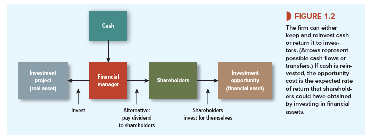
OK, let’s take the objective as maximizing market value. But why do some investments increase market value, while others reduce it? The answer is given by Figure 1.2, which sets out the fundamental trade-off for corporate investment decisions. Suppose the corporation has a proposed investment in a real asset and enough cash on hand to finance the investment. If the corporation does not invest, it can instead pay out the cash to shareholders—say, as an extra dividend. How does the financial manager decide whether to go ahead with the project or to pay out the cash? (The investment and dividend arrows in Figure 1.2 are arrows 2 and 4b in Figure 1.1.)
Assume that the financial manager is acting in the interests of the corporation’s owners, its stockholders. What do these stockholders want the financial manager to do? The answer depends on the project’s rate of return and on the rate of return that the stockholders can earn by investing in financial markets. If the return offered by the investment project is higher than shareholders can get by investing on their own, then the shareholders would vote for the investment project. If the investment project offers a lower return than shareholders can achieve on their own, they would vote to cancel the project and take the cash instead.
Perhaps the investment project in Figure 1.2 is a proposal for Tesla to launch a new electric car. Suppose Tesla has set aside cash to launch the new model in 2020. It could go ahead with the launch, or it could choose to cancel the investment and instead pay the cash out to its stockholders. If it pays out the cash, the stockholders can then invest for themselves.
Suppose that Tesla’s new project is just about as risky as the U.S. stock market and that investment in the stock market offers a 10% expected rate of return. If the project offers a superior rate of return—say, 20%—then Tesla’s stockholders would be happy for the company to keep the cash and invest it in the new model. If the project offers only a 5% return, then the stockholders are better off with the cash and without the new model; in that case, the financial manager should turn down the project.
As long as a corporation’s proposed investments offer higher rates of return than its shareholders can earn for themselves in the stock market (or in other financial markets), its shareholders will applaud the investments, and its stock price will increase. But if the company earns an inferior return, shareholders boo, stock price falls, and stockholders demand their money back so that they can invest on their own.
In our example, the minimum acceptable rate of return on Tesla’s new car is 10%. This minimum rate of return is called a hurdle rate or cost of capital. It is really an opportunity cost of capital because it depends on the investment opportunities available to investors in financial markets. Whenever a corporation invests cash in a new project, its shareholders lose the opportunity to invest the cash on their own. Corporations increase value by accepting all investment projects that earn more than the opportunity cost of capital.
Notice that the opportunity cost of capital depends on the risk of the proposed investment project. Why? It’s not just because shareholders are risk-averse. It’s also because shareholders have to trade off risk against return when they invest on their own. The safest investments, such as U.S. government debt, offer low rates of return. Investments with higher expected rates of return—the stock market, for example—are riskier and sometimes deliver painful losses. (The U.S. stock market was down 38% in 2008, for example.) Other investments are riskier still. For example, high-tech growth stocks offer the prospect of higher rates of return but are even more volatile.
Also notice that the opportunity cost of capital is generally not the interest rate that the company pays on a loan from a bank. If the company is making a risky investment, the opportunity cost is the expected return that investors can achieve in financial markets at the same level of risk. The expected return on risky securities is well above the interest rate on a bank loan.
Managers look to the financial markets to measure the opportunity cost of capital for the firm’s investment projects. They can observe the opportunity cost of capital for safe investments by looking up current interest rates on safe debt securities. For risky investments, the opportunity cost of capital has to be estimated. We start to tackle this task in Chapter 7.
4. Should Managers Look After the Interests of Their Shareholders?
So far we have assumed that financial managers should act on behalf of shareholders by trying to maximize their wealth. But perhaps this begs the questions: Is it desirable for managers to act in the selfish interests of their shareholders? Does a focus on enriching the shareholders mean that managers must act as greedy mercenaries riding roughshod over the weak and helpless?
Most of this book is devoted to financial policies that increase value. None of these policies requires gallops over the weak and helpless. In most instances, little conflict arises between doing well (maximizing value) and doing good. Profitable firms are those with satisfied customers and loyal employees; firms with dissatisfied customers and a disgruntled workforce will probably end up with declining profits and a low stock price.
Most established corporations can add value by building long-term relationships with their customers and establishing a reputation for fair dealing and financial integrity. When something happens to undermine that reputation, the costs can be enormous.
So, when we say that the objective of the firm is to maximize shareholder wealth, we do not mean that anything goes. The law deters managers from making blatantly dishonest decisions, but most managers should not be simply concerned with observing the letter of the law or with keeping to written contracts. In business and finance, as in other day-to-day affairs, there are unwritten rules of behavior. These rules make routine financial transactions feasible because each party to the transaction has to trust the other to keep to his or her side of the bargain.[2]
When something happens to damage that trust, the costs can be enormous. Volkswagen (VW) is a case in point. VW had installed secret software that cut back pollution from its diesel cars, but only when the cars were tested. Discovery of the software in 2015 caused a tidal wave of opprobrium. VW’s stock price dropped by 35%. Its CEO was fired. VW diesel vehicles piled up unsold in car dealers’ lots. In the United States alone, the scandal is likely to cost the company more than $20 billion in fines and compensation payments.
Charlatans and swindlers are often able to hide behind booming markets. It is only “when the tide goes out that you learn who’s been swimming naked.”7 The tide went out in 2008, and a number of frauds were exposed. One notorious example was the Ponzi scheme run by the New York financier Bernard Madoff.8 Individuals and institutions put about $65 billion in the scheme before it collapsed in 2008. (It’s not clear what Madoff did with all this money, but much of it was apparently paid out to early investors in the scheme to create an impression of superior investment performance.) With hindsight, the investors should not have trusted Madoff or the financial advisers who steered money to Madoff.
Madoff’s Ponzi scheme was (we hope) a once-in-a-lifetime event.9 It was astonishingly unethical, illegal, and bound to end in tears. That much is obvious. The difficult ethical problems for financial managers lurk in the grey areas. Look, for example, at the nearby Finance in Practice box that presents three ethical problems. Think about where you stand on these issues and where you would draw the ethical red line.
What is the underlying source of unethical business behavior? Sometimes it is simply because an employee is dishonest. But frequently the behavior stems from a culture in the firm that encourages high-pressure selling or unscrupulous dealing. In this case, the root of the problem lies with top management that promotes such values. (Click on the nearby Beyond the Page feature for an interesting demonstration of this in the banking industry.)
5. Agency Problems and Corporate Governance
We have emphasized the separation of ownership and control in public corporations. The owners (shareholders) cannot control what the managers do, except indirectly through the board of directors. This separation is necessary but also dangerous. You can see the risks. Managers may be tempted to buy sumptuous corporate jets or to schedule business meetings at tony resorts. They may shy away from attractive but risky projects because they are worried more about the safety of their jobs than about maximizing shareholder value. They may work just to maximize their own bonuses, and therefore redouble their efforts to make and resell flawed subprime mortgages.
Conflicts between shareholders’ and managers’ objectives create agency problems. Agency problems arise when agents work for principals. The shareholders are the principals; the managers are their agents. Agency costs are incurred when (1) managers do not attempt to maximize firm value and (2) shareholders incur costs to monitor the managers and constrain their actions.
Agency problems can sometimes lead to outrageous behavior. For example, when Dennis Kozlowski, the CEO of Tyco, threw a $2 million 40th birthday bash for his wife, he charged half of the cost to the company. This of course was an extreme conflict of interest, as well as illegal. But more subtle and moderate agency problems arise whenever managers think just a little less hard about spending money when it is not their own.
Later in the book we will look at how good systems of governance ensure that shareholders’ pockets are close to the managers’ hearts. This means well-designed incentives for managers, standards for accounting and disclosure to investors, requirements for boards of directors, and legal sanctions for self-dealing by management. When scandals happen, we say that corporate governance has broken down. When corporations compete effectively and ethically to deliver value to shareholders, we are comforted that governance is working properly.
Source: Brealey Richard A., Myers Stewart C., Allen Franklin (2020), Principles of Corporate Finance, McGraw-Hill Education; 13th edition.
The post The Financial Goal of the Corporation appeared first on HKT Consultant.
]]>The post Fintech and the Changing World of Finance appeared first on HKT Consultant.
]]>Payment Systems Not that many years ago, cash or checks were the principal way to pay for purchases, but in many countries, cash is fast disappearing. For example, in Sweden cash transactions make up barely 2% of the value of all payments. You can’t use cash to buy a bus ticket or a ticket on the Stockholm metro, and retailers are not legally obliged to accept coins and notes. The majority of Sweden’s bank branches no longer keep cash on hand or take cash deposits— and many branches no longer have ATMs. Instead of cash, Swedes use either a card or a mobile phone app to transfer money from one bank account to another in real time.
Peer-to-Peer (P2P) Lending Peer-to-peer lending platforms directly link individuals willing to lend money with people seeking to borrow. For example, in the United States would-be borrowers can apply to Lending Club for a personal loan of up to $40,000 or a business loan of up to $300,000. The company then assigns a credit score to that customer, and on the basis of this score, potential investors can choose whether to participate in the loan. Thus, Lending Club cuts banks out of the lending equation entirely. It does not lend itself; instead, it verifies the identity of borrowers and lenders, uses the credit score to set the interest rate for the loan, and services the loan.
Robo Advice Providing investment advice to individuals and tailoring portfolios to their particular needs can be a costly business. Robo advisers seek to reduce these costs by automating the process. You will first need to complete an online questionnaire describing your personal situation and your risk tolerance. The robo adviser will then recommend a portfolio, usually a basket of low-cost funds. Then, once you deposit money in the account, the robo adviser will buy the investments and rebalance your portfolio to maintain your ideal mix of assets.
Blockchains A blockchain consists of a network of computers that simultaneously update a ledger of transactions or other data. This ledger doesn’t exist in one place but is distributed across many participants in the network. Many believe that the technology offers a major advance in the speed and security of financial record-keeping. Stock exchanges around the world have begun to experiment with blockchains as a method for companies to list and trade their shares, and to ballot their shareholders. The effect should be lower costs of trading, faster transfers of ownership, and more accurate records.
Source: Brealey Richard A., Myers Stewart C., Allen Franklin (2020), Principles of Corporate Finance, McGraw-Hill Education; 13th edition.
The post Fintech and the Changing World of Finance appeared first on HKT Consultant.
]]>The post Future Values and Present Values appeared first on HKT Consultant.
]]>Money can be invested to earn interest. So, if you are offered the choice between $100 today and $100 next year, you naturally take the money now to get a year’s interest. Financial managers make the same point when they say that money has a time value or when they quote the most basic principle of finance: A dollar today is worth more than a dollar tomorrow.
Suppose you invest $100 in a bank account that pays interest of r = 7% a year. In the first year, you will earn interest of .07 X $100 = $7 and the value of your investment will grow to $107:
Value of investment after 1 year = $100 X (1 + r) = 100 X 1.07 = $107
By investing, you give up the opportunity to spend $100 today, but you gain the chance to spend $107 next year.
If you leave your money in the bank for a second year, you earn interest of .07 X $107 = $7.49 and your investment will grow to $114.49:
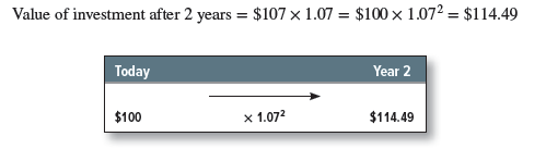
Notice that in the second year you earn interest on both your initial investment ($100) and the previous year’s interest ($7). Thus your wealth grows at a compound rate and the interest that you earn is called compound interest.
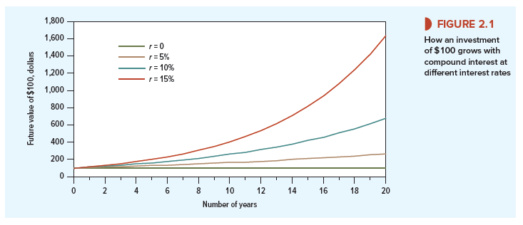
If you invest your $100 for t years, your investment will continue to grow at a 7% compound rate to $100 X (1.07/. For any interest rate r, the future value of your $100 investment will be
Future value of $100 = $100 X (1 + r)t
The higher the interest rate, the faster your savings will grow. Figure 2.1 shows that a few percentage points added to the interest rate can do wonders for your future wealth. For example, by the end of 20 years, $100 invested at 10% will grow to $100 X (1.10)20 = $672.75. If it is invested at 5%, it will grow to only $100 X (1.05)20 = $265.33.
2. Calculating Present Values
We have seen that $100 invested for two years at 7% will grow to a future value of 100 X 1.072 = $114.49. Let’s turn this around and ask how much you need to invest today to produce $114.49 at the end of the second year. In other words, what is the present value (PV) of the $114.49 payoff?
You already know that the answer is $100. But, if you didn’t know or you forgot, you can just run the future value calculation in reverse and divide the future payoff by (1.07)2:
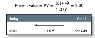
In general, suppose that you will receive a cash flow of Ct dollars at the end of year t. The present value of this future payment is
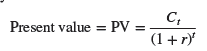
The rate, r, in the formula is called the discount rate, and the present value is the discounted value of the cash flow, Ct. You sometimes see this present value formula written differently. Instead of dividing the future payment by (1 + r)t, you can equally well multiply the payment by 1/(1 + r)t. The expression 1/(1 + r)t is called the discount factor. It measures the present value of one dollar received in year t. For example, with an interest rate of 7% the two-year discount factor is
DF2 = 1/(1.07)2 = .8734
Investors are willing to pay $.8734 today for delivery of $1 at the end of two years. If each dollar received in year 2 is worth $.8734 today, then the present value of your payment of $114.49 in year 2 must be
Present value = DF2 x C2 = .8734 x 114.49 = $100
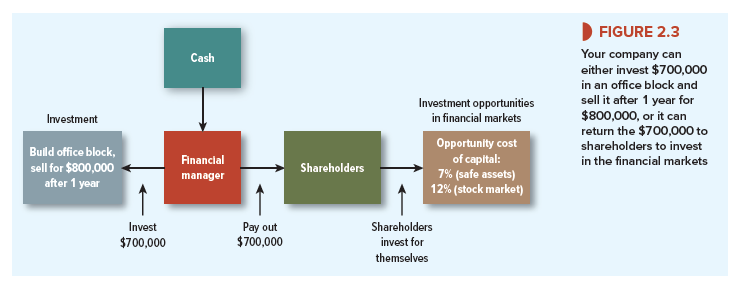
The longer you have to wait for your money, the lower its present value. This is illustrated in Figure 2.2. Notice how small variations in the interest rate can have a powerful effect on the present value of distant cash flows. At an interest rate of 5%, a payment of $100 in year 20 is worth $37.69 today. If the interest rate increases to 10%, the value of the future payment falls by about 60% to $14.86.
3. Valuing an Investment Opportunity
How do you decide whether an investment opportunity is worth undertaking? Suppose you own a small company that is contemplating construction of a suburban office block. The cost of buying the land and constructing the building is $700,000. Your company has cash in the bank to finance construction. Your real estate adviser forecasts a shortage of office space and predicts that you will be able to sell next year for $800,000. For simplicity, we will assume initially that this $800,000 is a sure thing.
The rate of return on this one-period project is easy to calculate. Divide the expected profit ($800,000 – 700,000 = $100,000) by the required investment ($700,000). The result is 100,000/700,000 = .143, or 14.3%.
Figure 2.3 summarizes your choices. (Note the resemblance to Figure 1.2 in the previous chapter.) You can invest in the project or pay cash out to shareholders, who can invest on their own. We assume that they can earn a 7% profit by investing for one year in safe assets (U.S. Treasury debt securities, for example). Or they can invest in the stock market, which is risky but offers an average return of 12%.
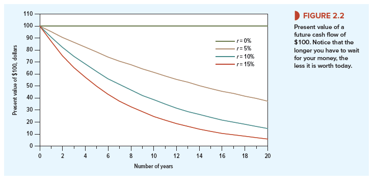
What is the opportunity cost of capital, 7% or 12%? The answer is 7%: That’s the rate of return that your company’s shareholders could get by investing on their own at the same level of risk as the proposed project. Here the level of risk is zero. (Remember, we are assuming for now that the future value of the office block is known with certainty.) Your shareholders would vote unanimously for the investment project because the project offers a safe return of 14% versus a safe return of only 7% in financial markets.
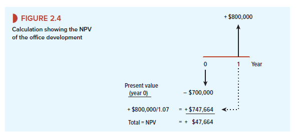
The office-block project is therefore a “go,” but how much is it worth and how much will the investment add to your wealth? The project produces a cash flow at the end of one year. To find its present value we discount that cash flow by the opportunity cost of capital:

Suppose that as soon as you have bought the land and paid for the construction, you decide to sell your project. How much could you sell it for? That is an easy question. If the venture will return a surefire $800,000, then your property ought to be worth its PV of $747,664 today.
That is what investors in the financial markets would need to pay to get the same future payoff. If you tried to sell it for more than $747,664, there would be no takers because the property would then offer an expected rate of return lower than the 7% available on government securities. Of course, you could always sell your property for less, but why sell for less than the market will bear? The $747,664 present value is the only feasible price that satisfies both buyer and seller. Therefore, the present value of the property is also its market price.
4. Net Present Value
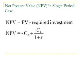
The office building is worth $747,664 today, but that does not mean you are $747,664 better off. You invested $700,000, so the net present value (NPV) is $47,664. Net present value equals present value minus the required investment:
NPV = PV – investment = 747,664 – 700,000 = $47,664
In other words, your office development is worth more than it costs. It makes a net contribution to value and increases your wealth. The formula for calculating the NPV of your project can be written as:

Remember that C0, the cash flow at time 0 (that is, today) is usually a negative number. In other words, C0 is an investment and therefore a cash outflow. In our example, C0 = -$700,000.
When cash flows occur at different points in time, it is often helpful to draw a timeline showing the date and value of each cash flow. Figure 2.4 shows a timeline for your office development. It sets out the net present value calculation assuming that the discount rate r is 7%.1
5. Risk and Present Value
We made one unrealistic assumption in our discussion of the office development: Your real estate adviser cannot be certain about the profitability of an office building. Those future cash flows represent the best forecast, but they are not a sure thing.
If the cash flows are uncertain, your calculation of NPV is wrong. Investors could achieve those cash flows with certainty by buying $747,664 worth of U.S. government securities, so they would not buy your building for that amount. You would have to cut your asking price to attract investors’ interest.
Here we can invoke a second basic financial principle: A safe dollar is worth more than a risky dollar. Most investors dislike risky ventures and won’t invest in them unless they see the prospect of a higher return. However, the concepts of present value and the opportunity cost of capital still make sense for risky investments. It is still proper to discount the payoff by the rate of return offered by a risk-equivalent investment in financial markets. But we have to think of expected payoffs and the expected rates of return on other investments.[1]
Not all investments are equally risky. The office development is more risky than a government security but less risky than a start-up biotech venture. Suppose you believe the project is as risky as investment in the stock market and that stocks are expected to provide a 12% return. Then 12% is the opportunity cost of capital for your project. That is what you are giving up by investing in the office building and not investing in equally risky securities.
Now recompute NPV with r = .12:
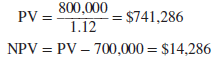
The office building still makes a net contribution to value, but the increase in your wealth is smaller than in our first calculation, which assumed that the cash flows from the project were risk-free.
The value of the office building depends, therefore, on the timing of the cash flows and their risk. The $800,000 payoff would be worth just that if you could get it today. If the office building is as risk-free as government securities, the delay in the cash flow reduces value by $52,336 to $747,664. If the building is as risky as investment in the stock market, then the risk further reduces value by $33,378 to $714,286.
Unfortunately, adjusting asset values for both time and risk is often more complicated than our example suggests. Therefore, we take the two effects separately. For the most part, we dodge the problem of risk in Chapters 2 through 6, either by treating all cash flows as if they were known with certainty or by talking about expected cash flows and expected rates of return without worrying how risk is defined or measured. Then in Chapter 7 we turn to the problem of understanding how financial markets cope with risk.
6. Present Values and Rates of Return
We have decided that constructing the office building is a smart thing to do since it is worth more than it costs. To discover how much it is worth, we asked how much you would need to invest directly in securities to achieve the same payoff. That is why we discounted the project’s future payoff by the rate of return offered by these equivalent-risk securities—the overall stock market in our example.
We can state our decision rule in another way: Your real estate venture is worth undertaking because its rate of return exceeds the opportunity cost of capital. The rate of return is simply the profit as a proportion of the initial outlay:

The cost of capital is once again the return foregone by not investing in financial markets. If the office building is as risky as investing in the stock market, the return foregone is 12%.
Since the 14.3% return on the office building exceeds the 12% opportunity cost, you should go ahead with the project.
Building the office block is a smart thing to do, even if the payoff is just as risky as the stock market. We can justify the investment by either one of the following two rules:3
- Net present value rule. Accept investments that have positive net present values.
- Rate of return rule. Accept investments that offer rates of return in excess of their opportunity costs of capital.
Properly applied, both rules give the same answer, although we will encounter some cases in Chapter 5 where the rate of return rule is easily misused. In those cases, it is safest to use the net present value rule.
7. Calculating Present Values When There Are Multiple Cash Flows
One of the nice things about present values is that they are all expressed in current dollars—so you can add them up. In other words, the present value of cash flow (A + B) is equal to the present value of cash flow A plus the present value of cash flow B.

Suppose that you wish to value a stream of cash flows extending over a number of years. Our rule for adding present values tells us that the total present value is:

This is called the discounted cash flow (or DCF) formula. A shorthand way to write it is
where £ refers to the sum of the series of discounted cash flows. To find the net present value (NPV) we add the (usually negative) initial cash flow:

Example 2.1 • Present Values with Multiple Cash Flows
Your real estate adviser has come back with some revised forecasts. He suggests that you rent out the building for two years at $30,000 a year, and predicts that at the end of that time you will be able to sell the building for $840,000. Thus there are now two future cash flows—a cash flow of C1 = $30,000 at the end of one year and a further cash flow of C2 = (30,000 + 840,000) = $870,000 at the end of the second year.
The present value of your property development is equal to the present value of C1 plus the present value of C2. Figure 2.5 shows that the value of the first year’s cash flow is Ci/(1 + r) = 30,000/1.12 = $26,786 and the value of the second year’s flow is C2/(1 + r)2 = 870,000/1.122 = $693,559. Therefore our rule for adding present values tells us that the total present value of your investment is:

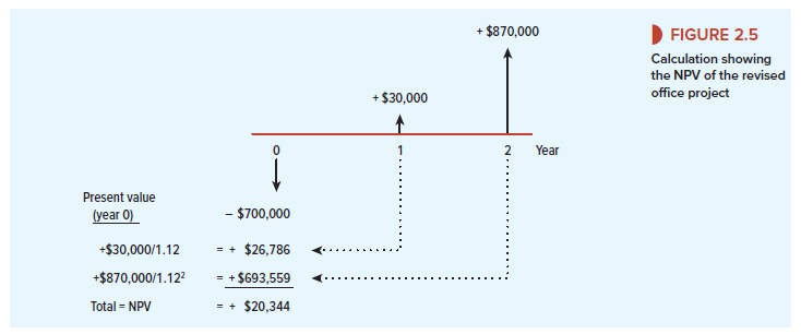
It looks as if you should take your adviser’s suggestion. NPV is higher than if you sell in year 1: NPV = $720,344 – $700,000 = $20,344
Your two-period calculations in Example 2.1 required just a few keystrokes on a calculator. Real problems can be much more complicated, so financial managers usually turn to financial calculators especially programmed for present value calculations or to computer spreadsheet programs. A box near the end of the chapter introduces you to some useful Excel functions that can be used to solve discounting problems.
8. The Opportunity Cost of Capital
By investing in the office building you are giving up the opportunity to earn an expected return of 12% in the stock market. The opportunity cost of capital is therefore 12%. When you discount the expected cash flows by the opportunity cost of capital, you are asking how much investors in the financial markets are prepared to pay for a security that produces a similar stream of future cash flows. Your calculations showed that these investors would need to pay $720,344 for an investment that produces cash flows of $30,000 at year 1 and $870,000 at year 2. Therefore, they won’t pay any more than that for your office building.
Confusion sometimes sneaks into discussions of the cost of capital. Suppose a banker approaches. “Your company is a fine and safe business with few debts,” she says. “My bank will lend you the $700,000 that you need for the office block at 8%.” Does this mean that the cost of capital is 8%? If so, the project would be even more worthwhile. At an 8% cost of capital, PV would be 30,000/1.08 + 870,000/1.082 = $773,663 and NPV = $773,663 – $700,000 = +$73,663.
But that can’t be right. First, the interest rate on the loan has nothing to do with the risk of the project: it reflects the good health of your existing business. Second, whether you take the loan or not, you still face the choice between the office building and an equally risky investment in the stock market. A financial manager who borrows $700,000 at 8% and invests in an office building is not smart, but stupid, if the company or its shareholders can borrow at 8% and make an equally risky investment in the stock market offering an even higher return. That is why the 12% expected return on the stock market is the opportunity cost of capital for your project.
Source: Brealey Richard A., Myers Stewart C., Allen Franklin (2020), Principles of Corporate Finance, McGraw-Hill Education; 13th edition.
The post Future Values and Present Values appeared first on HKT Consultant.
]]>The post Looking for Shortcuts – Perpetuities and Annuities appeared first on HKT Consultant.
]]>Sometimes there are shortcuts that make it easy to calculate present values. Let us look at some examples.
On occasion, the British and the French have been known to disagree and sometimes even to fight wars. At the end of some of these wars the British consolidated the debt they had issued during the war. The securities issued in such cases were called consols. Consols are perpetuities. They are bonds that the government is under no obligation to repay but that offer a fixed income for each year to perpetuity. The British government is still paying interest on consols issued all those years ago. The annual rate of return on a perpetuity is equal to the promised annual payment divided by the present value:
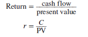
We can obviously twist this around and find the present value of a perpetuity given the discount rate r and the cash payment C:4
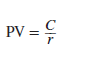
The year is 2030. You have been fabulously successful and are now a billionaire many times over. It was fortunate indeed that you took that finance course all those years ago. You have decided to follow in the footsteps of two of your philanthropic heroes, Bill Gates and Warren Buffett. Malaria is still a scourge and you want to help eradicate it and other infectious diseases by endowing a foundation to combat these diseases. You aim to provide $1 billion a year in perpetuity, starting next year. So, if the interest rate is 10%, you need to write a check today for

Two warnings about the perpetuity formula. First, at a quick glance, you can easily confuse the formula with the present value of a single payment. A payment of $1 at the end of one year has a present value of 1/(1 + r). The perpetuity has a value of 1/r. These are quite different.
Second, the perpetuity formula tells us the value of a regular stream of payments starting one period from now. Thus your $10 billion endowment would provide the foundation with its first payment in one year’s time. If you also want to provide an up-front sum, you will need to lay out an extra $1 billion.

Sometimes you may need to calculate the value of a perpetuity that does not start to make payments for several years. For example, suppose that you decide to provide $1 billion a year with the first payment four years from now. Figure 2.6 provides a timeline of these payments. Think first about how much they will be worth in year 3. At that point the endowment will be an ordinary perpetuity with the first payment due at the end of the year. So our perpetuity formula tells us that in year 3 the endowment will be worth $1/r = $1/.1 = $10 billion. But it is not worth that much now. To find today’s value we need to multiply by the three-year discount factor 1/(1 + r)3 = 1/(1.1)3 = .751. Thus, the “delayed” perpetuity is worth $10 billion x .751 = $7.51 billion. The full calculation is:

2. How to Value Annuities
An annuity is an asset that pays a fixed sum each year for a specified number of years. The equal-payment house mortgage or installment credit agreement are common examples of annuities. So are interest payments on most bonds, as we shall see in the next chapter.
You can always value an annuity by calculating the value of each cash flow and finding the total. However, it is often quicker to use a simple formula that states that if the interest rate is r, then the present value of an annuity that pays $C a period for each of t periods is:

The expression in brackets shows the present value of $1 a year for each of t years. It is generally known as the t-year annuity factor.
If you are wondering where this formula comes from, look at Figure 2.7. It shows the payments and values of three investments.
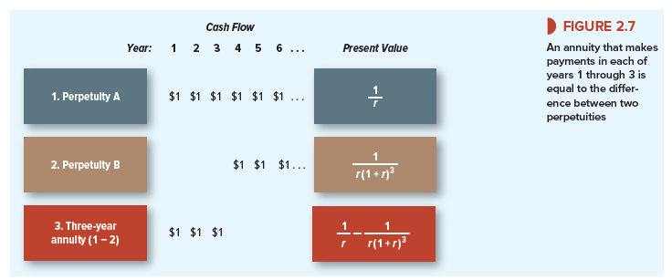
Row 1 The investment in the first row provides a perpetual stream of $1 starting at the end of the first year. We have already seen that this perpetuity has a present value of 1/r.
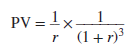
Row 2 Now look at the investment shown in the second row of Figure 2.7. It also provides a perpetual stream of $1 payments, but these payments don’t start until year 4. This stream of payments is identical to the payments in row 1, except that they are delayed for an additional three years. In year 3, the investment will be an ordinary perpetuity with payments starting in one year and will therefore be worth 1/r in year 3. To find the value today, we simply multiply this figure by the three-year discount factor. Thus, as we saw earlier
Row 3 Finally, look at the investment shown in the third row of Figure 2.7. This provides a level payment of $1 a year for each of three years. In other words, it is a three-year annuity. You can also see that, taken together, the investments in rows 2 and 3 provide exactly the same cash payments as the investment in row 1. Thus the value of our annuity (row 3) must be equal to the value of the row 1 perpetuity less the value of the delayed row 2 perpetuity:

Remembering formulas is about as difficult as remembering other people’s birthdays. But as long as you bear in mind that an annuity is equivalent to the difference between an immediate and a delayed perpetuity, you shouldn’t have any difficulty.5
Example 2.2 • Costing an Installment Plan
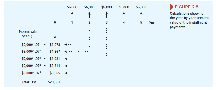
Most installment plans call for level streams of payments. Suppose that Tiburon Autos offers an “easy payment” scheme on a new Toyota of $5,000 a year, paid at the end of each of the next five years, with no cash down. What is the car really costing you?
First let us do the calculations the slow way, to show that if the interest rate is 7%, the present value of these payments is $20,501. The timeline in Figure 2.8 shows the value of each cash flow and the total present value. The annuity formula, however, is generally quicker; you simply need to multiply the $5,000 cash flow by the annuity factor:

3. Valuing Annuities Due
When we costed the installment plan we assumed that the first payment was made at the end of the year. Suppose instead that the first of the five yearly payments is due immediately. How does this change the cost of the car?
If we discount each cash flow by one less year, the present value is increased by the multiple (1 + r). In the case of the car purchase the present value of the payments becomes 20,501 X (1 + r) = 20,501 X 1.07 = $21,936.
A level stream of payments starting immediately is called an annuity due. An annuity due is worth (1 + r) times the value of an ordinary annuity.
4. Calculating Annual Payments
Annuity problems can be confusing on first acquaintance, but you will find that with practice they are generally straightforward. For example, here is a case where you need to use the annuity formula to find the amount of the payment given the present value.
Example 2.3 • Paying Off a Bank Loan
Bank loans are paid off in equal installments. Suppose that you take out a four-year loan of $1,000. The bank requires you to repay the loan evenly over the four years. It must therefore set the four annual payments so that they have a present value of $1,000. Thus,
PV = annual loan payment X 4-year annuity factor = $1,000
Annual loan payment = $1,000/4-year annuity factor
Suppose that the interest rate is 10% a year. Then
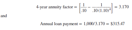
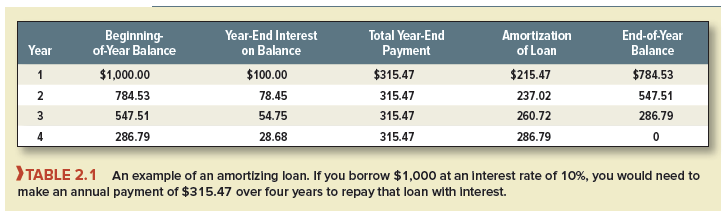
Let’s check that this annual payment is sufficient to repay the loan. Table 2.1 provides the calculations. At the end of the first year, the interest charge is 10% of $1,000, or $100. So $100 of the first payment is absorbed by interest, and the remaining $215.47 is used to reduce the loan balance to $784.53.
Next year, the outstanding balance is lower, so the interest charge is only $78.45. Therefore $315.47 – $78.45 = $237.02 can be applied to paying off the loan. Because the loan is progressively paid off, the fraction of each payment devoted to interest steadily falls over time, while the fraction used to reduce the loan increases. By the end of year 4, the amortization is just enough to reduce the balance of the loan to zero.
Loans that involve a series of level payments are known as amortizing loans. “Amortizing” means that part of the regular payment is used to pay interest on the loan and part is used to pay off or amortize the loan.
Example 2.4 • Calculating Mortgage Payments
Most mortgages are amortizing loans. For example, suppose that you take out a $250,000 house mortgage from your local savings bank when the interest rate is 12%. The bank requires you to repay the mortgage in equal annual installments over the next 30 years.
Thus,
Annual mortgage payment = $250,000/30-year annuity factor

and
Annual mortgage payment = 250,000/8.055 = $31,036
Figure 2.9 shows that in the early years, almost all of the mortgage payment is eaten up by interest and only a small fraction is used to reduce the amount of the loan. Even after 15 years, the bulk of the annual payment goes to pay the interest on the loan. From then on, the amount of the loan begins to decline rapidly.
Source: Brealey Richard A., Myers Stewart C., Allen Franklin (2020), Principles of Corporate Finance, McGraw-Hill Education; 13th edition.
The post Looking for Shortcuts – Perpetuities and Annuities appeared first on HKT Consultant.
]]>The post More Shortcuts – Growing Perpetuities and Annuities appeared first on HKT Consultant.
]]>You now know how to value level streams of cash flows, but you often need to value a stream of cash flows that grows at a constant rate. For example, think back to your plans to donate $10 billion to fight malaria and other infectious diseases. Unfortunately, you made no allowance for the growth in salaries and other costs, which will probably average about 4% a year starting in year 1. Therefore, instead of providing $1 billion a year in perpetuity, you must provide $1 billion in year 1, 1.04 x $1 billion in year 2, and so on. If we call the growth rate in costs g, we can write down the present value of this stream of cash flows as follows:
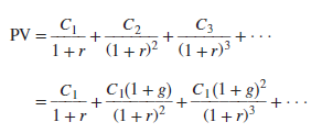
Fortunately, there is a simple formula for the sum of this geometric series.6 If we assume that r is greater than g, our clumsy-looking calculation simplifies to

Therefore, if you want to provide a perpetual stream of income that keeps pace with the growth rate in costs, the amount that you must set aside today is

You will meet this perpetual-growth formula again in Chapter 4, where we use it to value the stocks of mature, slowly growing companies.
2. Growing Annuities
Example 2.6 • Winning Big at the Lottery
In August 2017, a Massachusetts woman invested in a Powerball lottery ticket and won a record $758.7 million. We suspect that she received unsolicited congratulations, good wishes, and requests for money from dozens of more or less worthy charities, relations, and newly devoted friends. In response, she could fairly point out that the prize wasn’t really worth $758.7 million. That sum was to be paid in 30 annual installments. The payment in the first year was only $11.42 million, but it then increased each year by 5% so that the final payment was $47.00 million. The total amount paid out was $758.7 million, but the winner had to wait to get it.
If the interest rate was 2.7%, what was that $758.7 prize really worth? Suppose that the first payment occurs at the end of year 1, so that C1 = $11.42 million. If the payments then grow at the rate of g = .05 each year, the payment in year 2 is 11.42 x 1.05, and in year 3 it is 11.42 x 1.052. Of course, you could calculate each of the 30 cash flows and discount them at 2.7%. The alternative is to use the following formula for the present value of a growing annuity:

In the case of our lottery, the present value of the growing stream of payments is

Thus, the present value of a growing stream of payments starting at the end of the first year is $468 million. In practice, the news is not quite that bad because the lottery winner receives the first payment immediately (in year 0) and the last one is received in year 29 rather than in year 30. Therefore, we need to increase our estimate of present value by 1 + r. So the present value of the prize is 468 × 1.027 = $481 million.
If the total Powerball prize money was paid out immediately, it would be worth $757.8 million. Paying out this money over the next 29 years reduces the value of the prize to $481 million, much below the well-trumpeted prize but still not a bad day’s haul.
For winners with big spending plans, lottery operators generally make arrangements so that they may take an equivalent lump sum. In our example, the winner could either take the $758.7 million spread over 30 years or receive $481 million up front. Both arrangements had the same present value.
Too many formulas are bad for the digestions. So we will stop at this point and spare you any more of them. The formulas discussed so far appear in Table 2.2.
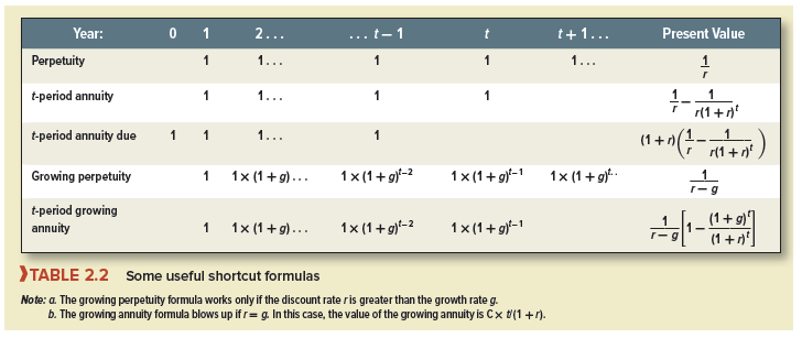
Source: Brealey Richard A., Myers Stewart C., Allen Franklin (2020), Principles of Corporate Finance, McGraw-Hill Education; 13th edition.
The post More Shortcuts – Growing Perpetuities and Annuities appeared first on HKT Consultant.
]]>The post How Interest Is Paid and Quoted appeared first on HKT Consultant.
]]>If the first interest payment is made at the end of six months, you can earn an additional six months’ interest on this payment. For example, if you invest $100 in a bond that pays interest of 10% compounded semiannually, your wealth will grow to 1.05 X $100 = $105 by the end of six months and to 1.05 X $105 = $110.25 by the end of the year. In other words, an interest rate of 10% compounded semiannually is equivalent to 10.25% compounded annually. The effective annual interest rate on the bond is 10.25%.
Let’s take another example. Suppose a bank offers you an automobile loan at an annual percentage rate, or APR, of 12% with interest to be paid monthly. By this the bank means that each month you need to pay one-twelfth of the annual rate, that is, 12/12 = 1% a month. Thus the bank is quoting a rate of 12%, but the effective annual interest rate on your loan is 1.0112 – 1 = .1268 or 12.68%.[1]
Our examples illustrate that you need to distinguish between the quoted annual interest rate and the effective annual rate. The quoted annual rate is usually calculated as the total annual payment divided by the number of payments in the year. When interest is paid once a year, the quoted and effective rates are the same. When interest is paid more frequently, the effective interest rate is higher than the quoted rate.
In general, if you invest $1 at a rate of r per year compounded m times a year, your investment at the end of the year will be worth [1 + (r/m)]m and the effective interest rate is [1 + (r/m)]m – 1. In our automobile loan example r = .12 and m = 12. So the effective annual interest rate was [1 + .12/12]12 – 1 = .1268, or 12.68%.
1. Continuous Compounding
Instead of compounding interest monthly or semiannually, the rate could be compounded weekly (m = 52) or daily (m = 365). In fact, there is no limit to how frequently interest could be paid. One can imagine a situation where the payments are spread evenly and continuously throughout the year, so the interest rate is continuously compounded.9 In this case m is infinite.
It turns out that there are many occasions in finance when continuous compounding is useful. For example, one important application is in option pricing models, such as the Black- Scholes model that we introduce in Chapter 21. These are continuous time models. So you will find that most computer programs for calculating option values ask for the continuously compounded interest rate.
It may seem that a lot of calculations would be needed to find a continuously compounded interest rate. However, think back to your high school algebra. You may recall that as m approaches infinity [1 + (r/m)]m approaches (2.718)r . The figure 2.718—or e, as it is called—is the base for natural logarithms. Therefore, $1 invested at a continuously compounded rate of r will grow to er = (2.718)r by the end of the first year. By the end of t years it will grow to ert = (2.718)rt.
Example 1 Suppose you invest $1 at a continuously compounded rate of 11% (r = .11) for one year (t = 1). The end-year value is e11, or $1.116. In other words, investing at 11% a year continuously compounded is exactly the same as investing at 11.6% a year annually compounded.
Example 2 Suppose you invest $1 at a continuously compounded rate of 11% (r = .11) for two years (t = 2). The final value of the investment is ert = e22, or $1.246.
Sometimes it may be more reasonable to assume that the cash flows from a project are spread evenly over the year rather than occurring at the year’s end. It is easy to adapt our previous formulas to handle this. For example, suppose that we wish to compute the present value of a perpetuity of C dollars a year. We already know that if the payment is made at the end of the year, we divide the payment by the annually compounded rate of r:

If the same total payment is made in an even stream throughout the year, we use the same formula but substitute the continuously compounded rate.
Suppose the annually compounded rate is 18.5%. The present value of a $100 perpetuity, with each cash flow received at the end of the year, is 100/.185 = $540.54. If the cash flow is received continuously, we must divide $100 by 17%, because 17% continuously compounded is equivalent to 18.5% annually compounded (e17 = 1.185). The present value of the continuous cash flow stream is 100/.17 = $588.24. Investors are prepared to pay more for the continuous cash payments because the cash starts to flow in immediately.
Example 3 After you have retired, you plan to spend $200,000 a year for 20 years. The annually compounded interest rate is 10%. How much must you save by the time you retire to support this spending plan?
Let us first do the calculations assuming that you spend the cash at the end of each year. In this case we can use the simple annuity formula that we derived earlier:

Thus, you will need to have saved $1.7 million by the time you retire.
Instead of waiting until the end of each year before you spend any cash, it is more reasonable to assume that your expenditure will be spread evenly over the year. In this case, instead of using the annually compounded rate of 10%, we must use the continuously compounded rate of r = 9.53% (e0953 = 1.10). Therefore, to cover a steady stream of expenditure, you need to set aside the following sum:[1]

To support a steady stream of outgoings, you must save an additional $83,600.
Often in finance you need only a ballpark estimate of present value. An error of 5% in a present value calculation may be perfectly acceptable. In such cases it doesn’t usually matter whether you assume that cash flows occur at the end of the year or in a continuous stream. At other times precision matters, and you do need to worry about the exact frequency of the cash flows.
Source: Brealey Richard A., Myers Stewart C., Allen Franklin (2020), Principles of Corporate Finance, McGraw-Hill Education; 13th edition.
The post How Interest Is Paid and Quoted appeared first on HKT Consultant.
]]>The post Using the Present Value Formula to Value Bonds appeared first on HKT Consultant.
]]>1. A Short Trip to Paris to Value a Government Bond
Why are we going to Paris, apart from the cafes, restaurants, and sophisticated nightlife? Because we want to start with the simplest type of bond, one that makes payments just once a year.
French government bonds, known as OATs (short for Obligations Assimilables du Tresor), pay interest and principal in euros (€). Suppose that in October 2017 you decide to buy €100 face value of the 6.00% OAT maturing in October 2025. Each year until the bond matures, you are entitled to an interest payment of .06 X 100 = €6.00. This amount is the bond’s coupon.1 When the bond matures in 2025, the government pays you the final €6.00 interest, plus the principal payment of €100. Your first coupon payment is in one year’s time, in October 2018. So the cash payments from the bond are as follows:
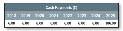
What is the present value of these payments? It depends on the opportunity cost of capital, which in this case equals the rate of return offered by other government debt issues denominated in euros. In October 2017, other medium-term French government bonds offered a return of just .3%. That is what you were giving up when you bought the 6.00% OATs. Therefore, to value the 6.00% OATs, you must discount the cash flows at .3%:

Bond prices are usually expressed as a percentage of face value. Thus the price of your 6.00% OAT was quoted as 144.99%.
You may have noticed a shortcut way to value this bond. Your OAT amounts to a package of two investments. The first investment gets the eight annual coupon payments of €6.00 each. The second gets the €100 face value at maturity. You can use the annuity formula from Chapter 2 to value the coupon payments and then add on the present value of the final payment.

Thus, the bond can be valued as a package of an annuity (the coupon payments) and a single, final payment (the repayment of principal).2
We just used the .3% interest rate to calculate the present value of the OAT. Now we turn the valuation around: If the price of the OAT is 144.99%, what is the interest rate? What return do investors get if they buy the bond and hold it to maturity? To answer this question, you need to find the value of the variable y that solves the following equation:

The rate of return y is called the bond’s yield to maturity. In this case, we already know that the present value of the bond is 144.99% at a .3% discount rate, so the yield to maturity must be .3%. If you buy the bond at 144.99% and hold it to maturity, you will earn a return of .3% per year.
Why is the yield to maturity less than the 6.00% coupon payment? Because you are paying €144.99 for a bond with a face value of only €100. You lose the difference of €44.99 if you hold the bond to maturity. On the other hand, you get eight annual cash payments of €6.00. (The immediate, current yield on your investment is 6.00/144.99 = .0414, or 4.14%.) The yield to maturity blends the return from the coupon payments with the declining value of the bond over its remaining life.
Let’s generalize. A bond, such as our OAT, that is priced above its face value is said to sell at a premium. Investors who buy a bond at a premium face a capital loss over the life of the bond, so the yield to maturity on these bonds is always less than the current yield. A bond that is priced below face value sells at a discount. Investors in discount bonds look forward to a capital gain over the life of the bond, so the yield to maturity on a discount bond is greater than the current yield.
The only general procedure for calculating the yield to maturity is trial and error. You guess at an interest rate and calculate the present value of the bond’s payments. If the present value is greater than the actual price, your discount rate must have been too low, and you need to try a higher rate. The more practical solution is to use a spreadsheet program or a specially programmed calculator to calculate the yield. At the end of this chapter, you will find a box that lists the Excel function for calculating yield to maturity plus several other useful functions for bond analysts.
2. Back to the United States: Semiannual Coupons and Bond Prices
Just like the French government, the U.S. Treasury raises money by regular auctions of new bond issues. Some of these issues do not mature for 20 or 30 years; others, known as notes, mature in 10 years or less. The Treasury also issues short-term debt maturing in a year or less. These short-term securities are known as Treasury bills. Treasury bonds, notes, and bills are traded in the fixed-income market.
Let’s look at an example of a U.S. government bond. In 1991, the Treasury issued 8.00% bonds maturing in 2021. These bonds are called “the 8s of 2021.” Treasury bonds and notes have face values of $1,000, so if you own the 8s of 2021, the Treasury will give you back $1,000 at maturity. You can also look forward to a regular coupon, but in contrast to our French bond, coupons on Treasury bonds and notes are paid semiannually.3 Thus, the 8s of 2021 provide a coupon payment of 8/2 = 4% of face value every six months.
You can’t buy Treasury bonds, notes, or bills on the stock exchange. They are traded by a network of bond dealers, who quote prices at which they are prepared to buy and sell. For example, suppose that you decide to buy the 8s of 2021. You phone a broker, who checks the current price on her screen. If you are happy to go ahead with the purchase, your broker contacts a bond dealer and the trade is done.
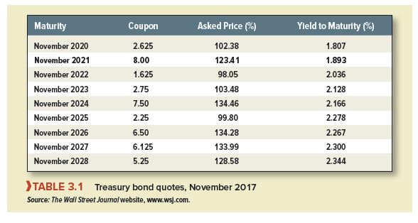
The prices at which you can buy or sell Treasury notes and bonds are shown each day in the financial press and on the web. In November 2017, there were 310 different Treasury notes and bonds. Table 3.1 shows the prices of just a small sample of them. Look at the entry for our 8.00s of 2021. The asked price, 123.41, is the price you need to pay to buy the bond from a dealer. This means that the 8.00% bond costs 123.41% of face value. The face value of the bond is $1,000, so each bond costs $1,234.10.[4]
The final column in the table shows the yield to maturity. Because interest is semiannual, annual yields on U.S. bonds are usually quoted as twice the semiannual yields. Thus, if you buy the 8.00% bond at the asked price and hold it to maturity, every six months you earn a return of 1.893/2 = .947%.
You can now repeat the present value calculations that we did for the French government bond. You just need to recognize that bonds in the U.S. have a face value of $1,000, that their coupons are paid semiannually, and that the quoted yield is a semiannually compounded rate.
Here are the cash payments for the 8.00s of 2021:

If investors demand a return of .947% every six months, then the present value of these cash flows is

Each bond is worth $1,234.10, or 123.41% of face value.
Again we could turn the valuation around: Given the price, what’s the yield to maturity? Try it, and you’ll find (no surprise) that the semiannual rate of return that you can earn over the eight remaining half-year periods is .00947. Take care to remember that the yield is reported as an annual rate, calculated as 2 x .00947 = .01893, or 1.893%. If you see a reported yield to maturity of R%, you have to remember to use y = R/2% as the semiannual rate for discounting cash flows received every six months.
Source: Brealey Richard A., Myers Stewart C., Allen Franklin (2020), Principles of Corporate Finance, McGraw-Hill Education; 13th edition.
The post Using the Present Value Formula to Value Bonds appeared first on HKT Consultant.
]]>The post How Bond Prices Vary with Interest Rates appeared first on HKT Consultant.
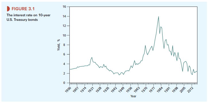
]]>
As interest rates change, so do bond prices. For example, suppose that investors demanded a semiannual return of 2% on the 8s of 2021, rather than the .947% semiannual return we used previously. In that case the price would be

The higher interest rate results in a lower price.
Bond prices and interest rates must move in opposite directions. The yield to maturity, our measure of the interest rate on a bond, is defined as the discount rate that explains the bond price. When bond prices fall, interest rates (i.e., yields to maturity) must rise. When interest rates rise, bond prices must fall. We recall a hapless TV pundit who intoned, “The recent decline in long-term interest rates suggests that long-term bond prices may rise over the next week or two.” Of course, the bond prices had already gone up. We are confident that you won’t make the pundit’s mistake.
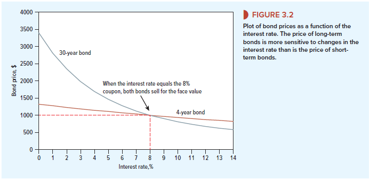
The brown line in Figure 3.2 shows the value of our 8% bond for different interest rates. As the yield to maturity falls, the bond price increases. When the annual yield is equal to the bond’s annual coupon rate (8%), the bond sells for exactly its face value. When the yield is higher than 8%, the bond sells at a discount to face value. When the yield is lower than 8%, the bond sells at a premium.
Bond investors cross their fingers that market interest rates will fall so that the price of their securities will rise. If they are unlucky and interest rates jump up, the value of their investment declines.
Example 3.1 • Changes in Interest Rates and Bond Returns
On May 15, 2008, the U.S. Treasury sold $9 billion of 4.375% bonds maturing in February 2038. The bonds were issued at a price of 96.38% and offered a yield to maturity of 4.60%. This was the return to anyone buying at the issue price and holding the bonds to maturity.
In the months following the issue, the financial crisis reached its peak. Lehman Brothers filed for bankruptcy with assets of $691 billion, and the government poured money into rescuing Fannie Mae, Freddie Mac, AIG, and a host of banks. As investors rushed to the safety of Treasury bonds, prices soared. By mid-December, the price of the 4.375s of 2038 had reached 138.05% of face value, and the yield had fallen to 2.5%. Anyone fortunate enough to have bought the bond at the issue price would have made a capital gain of $1,380.50 – $963.80 = $416.70. In addition, on August 15 the bond made its first coupon payment of $21.875 (this is the semiannual payment on the 4.375% coupon bond with a face value of $1,000). Our lucky investor would, therefore, have earned a seven-month rate of return of 45.5%:
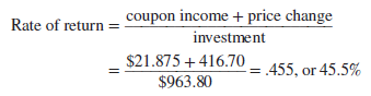
Suddenly, government bonds did not seem quite so boring as before.
A change in interest rates has only a modest impact on the value of near-term cash flows but a much greater impact on the value of distant cash flows. Thus the price of long-term bonds is affected more by changing interest rates than the price of short-term bonds. For example, compare the two curves in Figure 3.2. The brown line shows how the price of the four-year 8% bond varies with the interest rate. The blue line shows how the price of a 30-year 8% bond varies. You can see that the 30-year bond is much more sensitive to interest rate fluctuations than the four-year bond.
1. Duration and Volatility
Changes in interest rates have a greater impact on the prices of long-term bonds than on those of short-term bonds. But what do we mean by “long term” and “short term”? A coupon bond that matures in year 30 makes payments in each of years 1 through 30. It’s misleading to describe the bond as a 30-year bond; the average time to each cash payment is less than 30 years.
Example 3.2 • Which Is the Longer-Term Bond?
Table 3.2 calculates the prices of two seven-year bonds. We assume annual coupon payments and a yield to maturity of 4% per year. Take a look at the time pattern of each bond’s cash payments and review how the prices are calculated:
Which of these two bonds is the longer-term investment? They both have the same final maturity, of course. But the timing of the bonds’ cash payments is not the same. In the case of the 3s, the average time to each cash flow is longer, because a higher proportion of the cash flows occurs at maturity, when the face value is paid off.
Suppose now that the yield to maturity on each bond falls to 3%. Which bond would you most like to own? The 3s, of course. Since they have the longer effective life, they should benefit most from a fall in yields. Table 3.3 confirms that this is indeed the case:.
The 9s have the shorter average life and therefore a shift in interest rates has a more muted effect on the price. That much is clear. However, it would be useful to have a precise measure of the average life, one that could be used to predict the exposure of each bond’s price to fluctuations in interest rates. There is such a measure, and it is called duration or Macaulay duration after its founder.
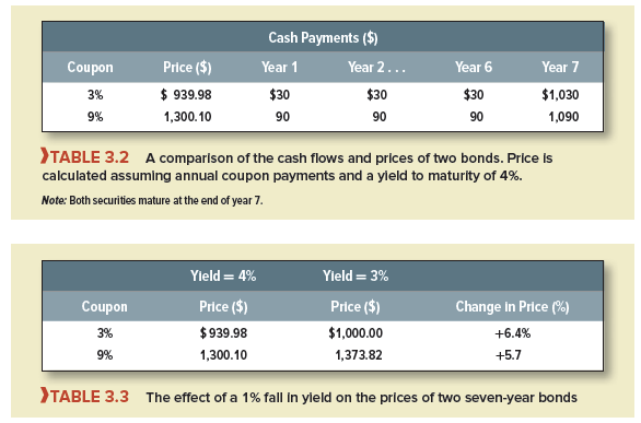
Duration is the weighted average of the times to each of the cash payments. The times are the future years 1, 2, 3, etc., extending to the final maturity date, which we call T. The weight for each year is the present value of the cash flow received at that time divided by the total present value of the bond.

Table 3.4 shows how to compute duration for the 9% seven-year bonds, assuming annual payments. First, we value each of the coupon payments of $90 and the final payment of coupon plus face value of $1,090. Of course, the present values of these payments add up to the bond price of $1,300.10. Then we calculate the fraction of the price accounted for by each cash flow and multiply each fraction by the year of the cash flow. The results sum across to a duration of 5.69 years.
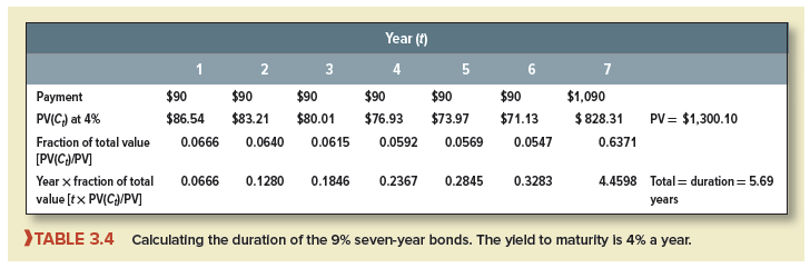
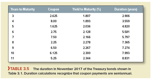
We leave it to you to calculate durations for the 3% bonds in Table 3.2. You will find that duration increases to 6.40 years.
Table 3.5 shows the duration in November 2017 of the sample of U.S. Treasury bonds set out in Table 3.1. Notice that, in all cases, the duration is shorter than the number of years to maturity and that the difference is most marked in the case of high coupon bonds.
We mentioned that investors and financial managers track duration because it measures how bond prices change when interest rates change. For this purpose, it’s best to use modified duration or volatility, which is just duration divided by one plus the yield to maturity:

Modified duration measures the percentage change in bond price for a 1 percentage-point change in yield.[2] Let’s try out this formula for our seven-year 9% bond in Table 3.3. The bond’s modified duration is duration/(1 + yield) = 5.69/1.04 = 5.47. This means that a 1% change in the yield to maturity should change the bond price by 5.47%.
Let’s check that prediction. Suppose the yield to maturity either increases or declines by .5%:
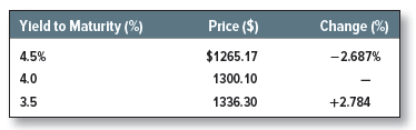
The total percentage difference between price at yields of 4.5% and 3.5% is 2.687 + 2.784 = 5.47%. Thus, a 1% change in interest rates means a 5.47% change in bond price, just as predicted.7
The modified duration for the 3% bond in Table 3.3 is 6.40/1.04 = 6.15%. In other words, a 1% change in yield to maturity results in a 6.15% change in the bond’s price. You can see why duration (or modified duration) is a handy measure of interest-rate risk.8
For example, the mini-case at the end of Chapter 26 looks at how financial managers can use the measure to protect the pension plan against unexpected changes in interest rates.
Source: Brealey Richard A., Myers Stewart C., Allen Franklin (2020), Principles of Corporate Finance, McGraw-Hill Education; 13th edition.
The post How Bond Prices Vary with Interest Rates appeared first on HKT Consultant.
]]>