The post Microeconomics: Introduction to Supply and Demand appeared first on HKT Consultant.
]]>While microeconomics focuses on firms and individuals, macroeconomics focuses on the sum total of economic activity, dealing with the issues of growth, inflation, and unemployment and with national policies relating to these issues. Microeconomics also deals with the effects of economic policies (such as changing taxation levels) on microeconomic behavior and thus on the aforementioned aspects of the economy. Particularly in the wake of the Lucas critique, much of modern macroeconomic theories has been built upon microfoundations—i.e. based upon basic assumptions about micro-level behavior.
Microeconomic theory typically begins with the study of a single rational and utility maximizing individual. To economists, rationality means an individual possesses stable preferences that are both complete and transitive. The technical assumption that preference relations are continuous is needed to ensure the existence of a utility function. Although microeconomic theory can continue without this assumption, it would make comparative statics impossible since there is no guarantee that the resulting utility function would be differentiable.
Main contentsSee more from basic to advanced


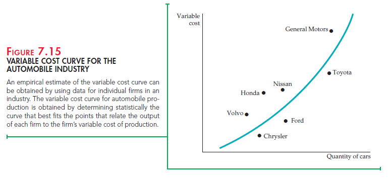


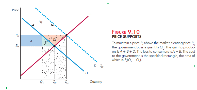
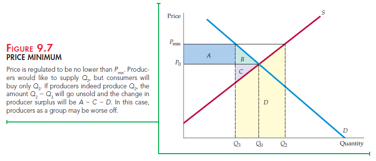

The post Microeconomics: Introduction to Supply and Demand appeared first on HKT Consultant.
]]>The post Introduction to Microeconomics appeared first on HKT Consultant.
]]>Much of microeconomics is about limits—the limited incomes that consumers can spend on goods and services, the limited budgets and technical know-how that firms can use to produce things, and the limited number of hours in a week that workers can allocate to labor or leisure. But microeconomics is also about ways to make the most of these limits. More precisely, it is about the allocation of scarce resources. For example, microeconomics explains how consumers can best allocate their limited incomes to the various goods and services available for purchase. It explains how workers can best allocate their time to labor instead of leisure, or to one job instead of another. And it explains how firms can best allocate limited financial resources to hiring additional workers versus buying new machinery, and to producing one set of products versus another.
In a planned economy such as that of Cuba, North Korea, or the former Soviet Union, these allocation decisions are made mostly by the government. Firms are told what and how much to produce, and how to produce it; workers have little flexibility in choice of jobs, hours worked, or even where they live; and consum- ers typically have a very limited set of goods to choose from. As a result, many of the tools and concepts of microeconomics are of limited relevance in those countries.
1. Trade–Offs
In modern market economies, consumers, workers, and firms have much more flexibility and choice when it comes to allocating scarce resources. Microeconomics describes the trade-offs that consumers, workers, and firms face, and shows how these trade-offs are best made.
The idea of making optimal trade-offs is an important theme in micro- economics—one that you will encounter throughout this book. Let’s look at it in more detail.
CONSUMERS Consumers have limited incomes, which can be spent on a wide variety of goods and services, or saved for the future. Consumer theory, the sub- ject matter of Chapters 3, 4, and 5 of this book, describes how consumers, based on their preferences, maximize their well-being by trading off the purchase of more of some goods for the purchase of less of others. We will also see how con- sumers decide how much of their incomes to save, thereby trading off current consumption for future consumption.
WORKERS Workers also face constraints and make trade-offs. First, people must decide whether and when to enter the workforce. Because the kinds of jobs—and corresponding pay scales—available to a worker depend in part on educational attainment and accumulated skills, one must trade off work- ing now (and earning an immediate income) for continued education (and the hope of earning a higher future income). Second, workers face trade-offs in their choice of employment. For example, while some people choose to work for large corporations that offer job security but limited potential for advancement, others prefer to work for small companies where there is more opportunity for advancement but less security. Finally, workers must sometimes decide how many hours per week they wish to work, thereby trading off labor for leisure.
FIRMS Firms also face limits in terms of the kinds of products that they can pro- duce, and the resources available to produce them. General Motors, for exam- ple, is very good at producing cars and trucks, but it does not have the ability to produce airplanes, computers, or pharmaceuticals. It is also constrained in terms of financial resources and the current production capacity of its factories. Given these constraints, GM must decide how many of each type of vehicle to produce. If it wants to produce a larger total number of cars and trucks next year or the year after, it must decide whether to hire more workers, build new factories, or do both. The theory of the firm, the subject matter of Chapters 6 and 7, describes how these trade-offs can best be made.
2. Prices and Markets
A second important theme of microeconomics is the role of prices. All of the trade-offs described above are based on the prices faced by consumers, workers, or firms. For example, a consumer trades off beef for chicken based partly on his or her preferences for each one, but also on their prices. Likewise, workers trade off labor for leisure based in part on the “price” that they can get for their labor—i.e., the wage. And firms decide whether to hire more workers or pur- chase more machines based in part on wage rates and machine prices.
Microeconomics also describes how prices are determined. In a centrally planned economy, prices are set by the government. In a market economy, prices are determined by the interactions of consumers, workers, and firms. These interactions occur in markets—collections of buyers and sellers that together determine the price of a good. In the automobile market, for example, car prices are affected by competition among Ford, General Motors, Toyota, and other manufacturers, and also by the demands of consumers. The central role of markets is the third important theme of microeconomics. We will say more about the nature and operation of markets shortly.
3. Theories and Models
Like any science, economics is concerned with the explanations of observed phenomena. Why, for example, do firms tend to hire or lay off workers when the prices of their raw materials change? How many workers are likely to be hired or laid off by a firm or an industry if the price of raw materials increases by, say,10 percent?
In economics, as in other sciences, explanation and prediction are based on theories. Theories are developed to explain observed phenomena in terms of a set of basic rules and assumptions. The theory of the firm, for example, begins with a simple assumption—firms try to maximize their profits. The theory uses this assumption to explain how firms choose the amounts of labor, capital, and raw materials that they use for production and the amount of output they produce.
It also explains how these choices depend on the prices of inputs, such as labor, capital, and raw materials, and the prices that firms can receive for their outputs. Economic theories are also the basis for making predictions. Thus the theory of the firm tells us whether a firm’s output level will increase or decrease in response to an increase in wage rates or a decrease in the price of raw materi- als. With the application of statistical and econometric techniques, theories can be used to construct models from which quantitative predictions can be made.
A model is a mathematical representation, based on economic theory, of a firm, a market, or some other entity. For example, we might develop a model of a par- ticular firm and use it to predict by how much the firm’s output level will change as a result of, say, a 10-percent drop in the price of raw materials.
Statistics and econometrics also let us measure the accuracy of our predictions. For example, suppose we predict that a 10-percent drop in the price of raw materi- als will lead to a 5-percent increase in output. Are we sure that the increase in out- put will be exactly 5 percent, or might it be somewhere between 3 and 7 percent? Quantifying the accuracy of a prediction can be as important as the prediction itself.
No theory, whether in economics, physics, or any other science, is perfectly correct. The usefulness and validity of a theory depend on whether it succeeds in explaining and predicting the set of phenomena that it is intended to explain and predict. Theories, therefore, are continually tested against observation. As a result of this testing, they are often modified or refined and occasionally even discarded. The process of testing and refining theories is central to the develop- ment of economics as a science.
When evaluating a theory, it is important to keep in mind that it is invariably imperfect. This is the case in every branch of science. In physics, for example, Boyle’s law relates the volume, temperature, and pressure of a gas.2 The law is based on the assumption that individual molecules of a gas behave as though they were tiny, elastic billiard balls. Physicists today know that gas molecules do not, in fact, always behave like billiard balls, which is why Boyle’s law breaks down under extremes of pressure and temperature. Under most conditions, however, it does an excellent job of predicting how the temperature of a gas will change when the pressure and volume change, and it is therefore an essential tool for engineers and scientists.
The situation is much the same in economics. For example, because firms do not maximize their profits all the time, the theory of the firm has had only limited success in explaining certain aspects of firms’ behavior, such as the timing of capital investment decisions. Nonetheless, the theory does explain a broad range of phenomena regarding the behavior, growth, and evolution of firms and indus- tries, and has thus become an important tool for managers and policymakers.
4. Positive versus Normative Analysis
Microeconomics is concerned with both positive and normative questions. Positive questions deal with explanation and prediction, normative questions with what ought to be. Suppose the U.S. government imposes a quota on the import of foreign cars. What will happen to the price, production, and sales of cars? What impact will this policy change have on American consumers? On workers in the automobile industry? These questions belong to the realm of positive analysis: statements that describe relationships of cause and effect.
Positive analysis is central to microeconomics. As we explained above, theories are developed to explain phenomena, tested against observations, and used to construct models from which predictions are made. The use of eco- nomic theory for prediction is important both for the managers of firms and for public policy. Suppose the federal government is considering raising the tax on gasoline. The change would affect the price of gasoline, consumers’ purchasing 2Robert Boyle (1627–1691) was a British chemist and physicist who discovered experimentally that pressure (P), volume (V), and temperature (T) were related in the following way: PV = RT, where R is a constant. Later, physicists derived this relationship as a consequence of the kinetic theory of gases, which describes the movement of gas molecules in statistical terms. choices for small or large cars, the amount of driving that people do, and so on. To plan sensibly, oil companies, automobile companies, producers of auto- mobile parts, and firms in the tourist industry would all need to estimate the impact of the change. Government policymakers would also need quantitative estimates of the effects. They would want to determine the costs imposed on consumers (perhaps broken down by income categories); the effects on profits and employment in the oil, automobile, and tourist industries; and the amount of tax revenue likely to be collected each year.
Sometimes we want to go beyond explanation and prediction to ask such questions as “What is best?” This involves normative analysis, which is also important for both managers of firms and those making public policy. Again, consider a new tax on gasoline. Automobile companies would want to deter- mine the best (profit-maximizing) mix of large and small cars to produce once the tax is in place. Specifically, how much money should be invested to make cars more fuel-efficient? For policymakers, the primary issue is likely to be whether the tax is in the public interest. The same policy objectives (say, an increase in tax revenues and a decrease in dependence on imported oil) might be met more cheaply with a different kind of tax, such as a tariff on imported oil.
Normative analysis is not only concerned with alternative policy options; it also involves the design of particular policy choices. For example, suppose it has been decided that a gasoline tax is desirable. Balancing costs and benefits, we then ask what is the optimal size of the tax.
Normative analysis is often supplemented by value judgments. For example, a comparison between a gasoline tax and an oil import tariff might conclude that the gasoline tax will be easier to administer but will have a greater impact on lower-income consumers. At that point, society must make a value judgment, weighing equity against economic efficiency. When value judgments are involved, microeconomics cannot tell us what the best policy is. However, it can clarify the trade-offs and thereby help to illuminate the issues and sharpen the debate.
Source: Pindyck Robert, Rubinfeld Daniel (2012), Microeconomics, Pearson, 8th edition.
The post Introduction to Microeconomics appeared first on HKT Consultant.
]]>The post What Is a Market? appeared first on HKT Consultant.
]]>It is easiest to understand what a market is and how it works by dividing individual economic units into two broad groups according to function—buyers and sellers. Buyers include consumers, who purchase goods and services, and firms, which buy labor, capital, and raw materials that they use to produce goods and services. Sellers include firms, which sell their goods and services; workers, who sell their labor services; and resource owners, who rent land or sell mineral resources to firms. Clearly, most people and most firms act as both buyers and sellers, but we will find it helpful to think of them as simply buyers when they are buying something and sellers when they are selling something.
Together, buyers and sellers interact to form markets. A market is the collection of buyers and sellers that, through their actual or potential interactions, determine the price of a product or set of products. In the market for personal computers, for example, the buyers are business firms, households, and students; the sellers are Hewlett-Packard, Lenovo, Dell, Apple, and a number of other firms. Note that a market includes more than an industry. An industry is a collection of firms that sell the same or closely related products. In effect, an industry is the supply side of the market.
Economists are often concerned with market definition—with determining which buyers and sellers should be included in a particular market. When defin- ing a market, potential interactions of buyers and sellers can be just as important as actual ones. An example of this is the market for gold. A New Yorker who wants to buy gold is unlikely to travel to Zurich to do so. Most buyers of gold in New York will interact only with sellers in New York. But because the cost of transporting gold is small relative to its value, buyers of gold in New York could purchase their gold in Zurich if the prices there were significantly lower.
Significant differences in the price of a commodity create a potential for arbitrage: buying at a low price in one location and selling at a higher price somewhere else. The possibility of arbitrage prevents the prices of gold in New York and Zurich from differing significantly and creates a world market for gold.
Markets are at the center of economic activity, and many of the most interest- ing issues in economics concern the functioning of markets. For example, why do only a few firms compete with one another in some markets, while in others a great many firms compete? Are consumers necessarily better off if there are many firms? If so, should the government intervene in markets with only a few firms? Why have prices in some markets risen or fallen rapidly, while in other markets prices have hardly changed at all? And which markets offer the best opportunities for an entrepreneur thinking of going into business?
1. Competitive versus Noncompetitive Markets
In this book, we study the behavior of both competitive and noncompetitive markets. A perfectly competitive market has many buyers and sellers, so that no single buyer or seller has any impact on price. Most agricultural markets are close to being perfectly competitive. For example, thousands of farmers produce wheat, which thousands of buyers purchase to produce flour and other prod- ucts. As a result, no single farmer and no single buyer can significantly affect the price of wheat.
Many other markets are competitive enough to be treated as if they were per- fectly competitive. The world market for copper, for example, contains a few dozen major producers. That number is enough for the impact on price to be small if any one producer goes out of business. The same is true for many other natural resource markets, such as those for coal, iron, tin, or lumber.
Other markets containing a small number of producers may still be treated as competitive for purposes of analysis. For example, the U.S. airline industry contains several dozen firms, but most routes are served by only a few firms. Nonetheless, because competition among those firms is often fierce, for some purposes airline markets can be treated as competitive. Finally, some markets contain many producers but are noncompetitive; that is, individual firms can jointly affect the price. The world oil market is one example. Since the early 1970s, that market has been dominated by the OPEC cartel. (A cartel is a group of producers that acts collectively.)
2. Market Price
Markets make possible transactions between buyers and sellers. Quantities of a good are sold at specific prices. In a perfectly competitive market, a single price—the market price—will usually prevail. The price of wheat in Kansas City and the price of gold in New York are two examples. These prices are usu- ally easy to measure. For example, you can find the price of corn, wheat, or gold each day in the business section of a newspaper.
In markets that are not perfectly competitive, different firms might charge different prices for the same product. This might happen because one firm is trying to win customers from its competitors, or because customers have brand loyalties that allow some firms to charge higher prices than others. For exam- ple, two brands of laundry detergent might be sold in the same supermarket at different prices. Or two supermarkets in the same town might sell the same brand of laundry detergent at different prices. In cases such as this, when we refer to the market price, we will mean the price averaged across brands or supermarkets.
The market prices of most goods will fluctuate over time, and for many goods the fluctuations can be rapid. This is particularly true for goods sold in competi- tive markets. The stock market, for example, is highly competitive because there are typically many buyers and sellers for any one stock. As anyone who has invested in the stock market knows, the price of any particular stock fluctuates from minute to minute and can rise or fall substantially during a single day. Likewise, the prices of commodities such as wheat, soybeans, coffee, oil, gold, silver, and lumber can rise or fall dramatically in a day or a week.
3. Market Definition—The Extent of a Market
As we saw, market definition identifies which buyers and sellers should be included in a given market. However, to determine which buyers and sellers to include, we must first determine the extent of a market—its boundaries, both geographically and in terms of the range of products to be included in it.
When we refer to the market for gasoline, for example, we must be clear about its geographic boundaries. Are we referring to downtown Los Angeles, south- ern California, or the entire United States? We must also be clear about the range of products to which we are referring. Should regular-octane and high-octane premium gasoline be included in the same market? Gasoline and diesel fuel?
For some goods, it makes sense to talk about a market only in terms of very restrictive geographic boundaries. Housing is a good example. Most people who work in downtown Chicago will look for housing within commuting dis- tance. They will not look at homes 200 or 300 miles away, even though those homes might be much cheaper. And homes (together with the land they are sitting on) 200 miles away cannot be easily moved closer to Chicago. Thus the housing market in Chicago is separate and distinct from, say, that in Cleveland, Houston, Atlanta, or Philadelphia. Likewise, retail gasoline markets, though less limited geographically, are still regional because of the expense of ship- ping gasoline over long distances. Thus the market for gasoline in southern California is distinct from that in northern Illinois. On the other hand, as we mentioned earlier, gold is bought and sold in a world market; the possibility of arbitrage prevents the price from differing significantly from one location to another.
We must also think carefully about the range of products to include in a market. For example, there is a market for single-lens reflex (SLR) digital cameras, and many brands compete in that market. But what about compact “point-and-shoot” digital cameras? Should they be considered part of the same market? Probably not, because they are typically used for different purposes and so do not compete with SLR cameras. Gasoline is another example. Regular- and premium-octane gasolines might be considered part of the same market because most consumers can use either. Diesel fuel, however, is not part of this market because cars that use regular gasoline cannot use diesel fuel, and vice versa.3
Market definition is important for two reasons:
- A company must understand who its actual and potential competitors are for the various products that it sells or might sell in the future. It must also know the product boundaries and geographical boundaries of its market in order to set price, determine advertising budgets, and make capital investment decisions.
- Market definition can be important for public policy decisions. Should the government allow a merger or acquisition involving companies that produce similar products, or should it challenge it? The answer depends on the impact of that merger or acquisition on future competition and prices; often this can be evaluated only by defining a market.
Source: Pindyck Robert, Rubinfeld Daniel (2012), Microeconomics, Pearson, 8th edition.
The post What Is a Market? appeared first on HKT Consultant.
]]>The post Real versus Nominal Prices appeared first on HKT Consultant.
]]>The nominal price of a good (sometimes called its “current-dollar” price) is its absolute price. For example, the nominal price of a pound of butter was about
$0.87 in 1970, $1.88 in 1980, about $1.99 in 1990, and about $3.42 in 2010. These are the prices you would have seen in supermarkets in those years. The real price of a good (sometimes called its “constant-dollar” price) is the price relative to an aggregate measure of prices. In other words, it is the price adjusted for inflation.
For consumer goods, the aggregate measure of prices most often used is the Consumer Price Index (CPI). The CPI is calculated by the U.S. Bureau of Labor Statistics by surveying retail prices, and is published monthly. It records how the cost of a large market basket of goods purchased by a “typical” consumer changes over time. Percentage changes in the CPI measure the rate of inflation in the economy.
Sometimes we are interested in the prices of raw materials and other interme- diate products bought by firms, as well as in finished products sold at wholesale to retail stores. In this case, the aggregate measure of prices often used is the Producer Price Index (PPI). The PPI is also calculated by the U.S. Bureau of Labor Statistics and published monthly, and records how, on average, prices at the wholesale level change over time. Percentage changes in the PPI measure cost inflation and predict future changes in the CPI.
So which price index should you use to convert nominal prices to real prices? It depends on the type of product you are examining. If it is a product or service normally purchased by consumers, use the CPI. If instead it is a product nor- mally purchased by businesses, use the PPI.
Because we are examining the price of butter in supermarkets, the relevant price index is the CPI. After correcting for inflation, do we find that the price of butter was more expensive in 2010 than in 1970? To find out, let’s calculate the
2010 price of butter in terms of 1970 dollars. The CPI was 38.8 in 1970 and rose to about 218.1 in 2010. (There was considerable inflation in the United States during the 1970s and early 1980s.) In 1970 dollars, the price of butter was
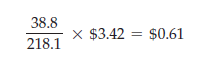
In real terms, therefore, the price of butter was lower in 2010 than it was in 1970.5. Put another way, the nominal price of butter went up by about 293 percent, while the CPI went up 462 percent. Relative to the aggregate price level, butter prices fell.
In this book, we will usually be concerned with real rather than nominal prices because consumer choices involve analyses of price comparisons. These relative prices can most easily be evaluated if there is a common basis of comparison. Stating all prices in real terms achieves this objective. Thus, even though we will often measure prices in dollars, we will be thinking in terms of the real purchas-ing power of those dollars.
Source: Pindyck Robert, Rubinfeld Daniel (2012), Microeconomics, Pearson, 8th edition.
The post Real versus Nominal Prices appeared first on HKT Consultant.
]]>The post Why Study Microeconomics? appeared first on HKT Consultant.
]]>1. Corporate Decision Making: The Toyota Prius
In 1997, Toyota Motor Corporation introduced the Prius in Japan, and started selling it worldwide in 2001. The Prius, the first hybrid car to be sold in the United States, can run off both a gasoline engine and a battery, and the momen- tum of the car charges the battery. Hybrid cars are more energy efficient than cars with just a gasoline engine; the Prius, for example, can get 45 to 55 miles per gallon. The Prius was a big success, and within a few years other manufacturers began introducing hybrid versions of some of their cars.
The design and efficient production of the Prius involved not only some impressive engineering, but a lot of economics as well. First, Toyota had to think carefully about how the public would react to the design and performance of this new product. How strong would demand be initially, and how fast would it grow? How would demand depend on the prices that Toyota charged? Understanding consumer preferences and trade-offs and predicting demand and its responsive- ness to price are essential to Toyota and every other automobile manufacturer. (We discuss consumer preferences and demand in Chapters 3, 4, and 5.)
Next, Toyota had to be concerned with the cost of manufacturing these cars — whether produced in Japan or, starting in 2010, in the United States. How high would production costs be? How would the cost of each car depend on the total number of cars produced each year? How would the cost of labor and the prices of steel and other raw materials affect costs? How much and how fast would costs decline as managers and workers gained experience with the production process? And to maximize profits, how many of these cars should Toyota plan to produce each year? (We discuss production and cost in Chapters 6 and 7, and the profit-maximizing choice of output in Chapters 8 and 10.)
Toyota also had to design a pricing strategy and consider how competitors would react to it. Although the Prius was the first hybrid car, Toyota knew that it would compete with other small fuel-efficient cars, and that soon other manufacturers would introduce their own hybrid cars. Should Toyota charge a relatively low price for a basic stripped-down version of the Prius and high prices for individual options like leather seats? Or would it be more profitable to make these options “standard” items and charge a higher price for the whole package? Whatever pricing strategy Toyota chose, how were competitors likely to react? Would Ford or Nissan try to undercut by lowering the prices of its smaller cars, or rush to bring out their own hybrid cars at lower prices? Might Toyota be able to deter Ford and Nissan from lowering prices by threatening to respond with its own price cuts? (We discuss pricing in Chapters 10 and 11, and competitive strategy in Chapters 12 and 13.)
Manufacturing the Prius required large investments in new capital equipment, so Toyota had to consider both the risks and possible outcomes of its decisions. Some of this risk was due to uncertainty over the future price of oil and thus the price of gasoline (lower gasoline prices would reduce the demand for small fuel- efficient cars). Some of the risk was due to uncertainty over the wages that Toyota would have to pay its workers at its plants in Japan and in the United States. (Oil and other commodity markets are discussed in Chapters 2 and 9. Labor markets and the impact of unions are discussed in Chapter 14. Investment decisions and the implications of uncertainty are discussed in Chapters 5 and 15.)
Toyota also had to worry about organizational problems. Toyota is an inte- grated firm in which separate divisions produce engines and parts and then assemble finished cars. How should the managers of different divisions be rewarded? What price should the assembly division be charged for the engines it receives from another division? (We discuss internal pricing and organiza- tional incentives for the integrated firm in Chapters 11 and 17.)
Finally, Toyota had to think about its relationship to the government and the effects of regulatory policies. For example, all of its cars sold in the United States must meet federal emissions standards, and U.S. production-line operations must comply with health and safety regulations. How might those regulations and standards change over time? How would they affect costs and profits? (We discuss the role of government in limiting pollution and promoting health and safety in Chapter 18.)
2. Public Policy Design: Fuel Efficiency Standards for the Twenty–First Century
In 1975, the U.S. government imposed regulations designed to improve the average fuel economy of domestically-sold cars and light trucks (including vans and sport utility vehicles). The CAFE (Corporate Average Fuel Economy) standards have become increasingly stringent over the years. In 2007, President George W. Bush signed into law the Energy Independence and Security Act, which required automakers to boost fleet wide gas mileage to 35 miles per gallon (mpg) by 2020. In 2011, the Obama administration pushed the 35 mpg target forward to 2016, and (with the agreement of 13 auto companies) set a standard of 55 mpg for 2020. While the program’s primary goal is to increase gas emissions.
A number of important decisions have to be made when designing a fuel efficiency program, and most of those decisions involve economics. First, the government must evaluate the monetary impact of the program on consumers. Higher fuel economy standards will increase the cost of purchasing a car (the cost of achieving higher fuel economy will be borne in part by consumers), but will lower the cost of operating it (gas mileage will be higher). Analyzing the ulti-mate impact on consumers means analyzing consumer preferences and demand. For example, would consumers drive less and spend more of their income on other goods? If so, would they be nearly as well off? (Consumer preferences and demand are discussed in Chapters 3 and 4).
Before imposing CAFE standards, it is important to estimate the likely impact those standards will have on the cost of producing cars and light trucks. Might automobile companies minimize cost increases by using new light-weight materials or by changing the footprint of new model cars? (Production and cost are discussed in Chapters 6 and 7.) Then the government needs to know how changes in production costs will affect the production levels and prices of new automobiles and light trucks. Are the additional costs likely to be absorbed by manufacturers or passed on to consumers in the form of higher prices? (Output determination is discussed in Chapter 8 and pricing in Chapters 10 through 13.)
The government must also ask why problems related to oil consumption are not solved by our market-oriented economy. One answer is that oil prices are determined in part by a cartel (OPEC) that is able to push the price of oil above competitive levels. (Pricing in markets in which firms have the power to control prices are discussed in Chapters 10 through 12.) Finally, the high U.S. demand for oil has led to a substantial outflow of dollars to the oil-producing countries, which in turn has created political and security issues that go beyond the con-fines of economics. What economics can do, however, is help us evaluate how best to reduce our dependence on foreign oil. Are standards like those of the CAFE program preferred to fees on oil consumption? What are the environ-mental implications of increasingly stringent standards? (These problems are discussed in Chapter 18.)
These are just two examples of how microeconomics can be applied in the arenas of private and public-policy decision making. You will discover many more applications as you read this book.
Source: Pindyck Robert, Rubinfeld Daniel (2012), Microeconomics, Pearson, 8th edition.
The post Why Study Microeconomics? appeared first on HKT Consultant.
]]>The post Supply and Demand appeared first on HKT Consultant.
]]>1. The Supply Curve
The supply curve shows the quantity of a good that producers are willing to sell at a given price, holding constant any other factors that might affect the quantity supplied. The curve labeled S in Figure 2.1 illustrates this. The vertical axis of the graph shows the price of a good, P, measured in dollars per unit. This is the price that sellers receive for a given quantity supplied. The horizontal axis shows the total quantity supplied, Q, measured in the number of units per period.
The supply curve is thus a relationship between the quantity supplied and the price. We can write this relationship as an equation:
QS = QS(P)
Or we can draw it graphically, as we have done in Figure 2.1.
Note that the supply curve in Figure 2.1 slopes upward. In other words, the higher the price, the more that firms are able and willing to produce and sell. For example, a higher price may enable current firms to expand production by hir-ing extra workers or by having existing workers work overtime (at greater cost to the firm). Likewise, they may expand production over a longer period of time by increasing the size of their plants. A higher price may also attract new firms to the market. These newcomers face higher costs because of their inex- perience in the market and would therefore have found entry uneconomical at a lower price.
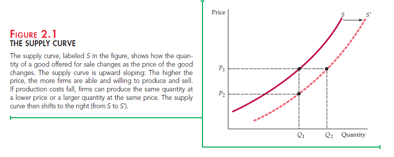
OTHER VARIABLES THAT AFFECT SUPPLY The quantity supplied can depend on other variables besides price. For example, the quantity that produc- ers are willing to sell depends not only on the price they receive but also on their production costs, including wages, interest charges, and the costs of raw materi- als. The supply curve labeled S in Figure 2.1 was drawn for particular values of these other variables. A change in the values of one or more of these variables translates into a shift in the supply curve. Let’s see how this might happen.
The supply curve S in Figure 2.1 says that at a price P1, the quantity produced and sold would be Q1. Now suppose that the cost of raw materials falls. How does this affect the supply curve?
Lower raw material costs—indeed, lower costs of any kind—make production more profitable, encouraging existing firms to expand production and enabling new firms to enter the market. If at the same time the market price stayed con- stant at P1, we would expect to observe a greater quantity supplied. Figure 2.1 shows this as an increase from Q1 to Q2. When production costs decrease, output increases no matter what the market price happens to be. The entire supply curve thus shifts to the right, which is shown in the figure as a shift from S to S’.
Another way of looking at the effect of lower raw material costs is to imag- ine that the quantity produced stays fixed at Q1 and then ask what price firms would require to produce this quantity. Because their costs are lower, they would accept a lower price—P2. This would be the case no matter what quantity was produced. Again, we see in Figure 2.1 that the supply curve must shift to the right.
We have seen that the response of quantity supplied to changes in price can be represented by movements along the supply curve. However, the response of supply to changes in other supply-determining variables is shown graphically as a shift of the supply curve itself. To distinguish between these two graphical depictions of supply changes, economists often use the phrase change in supply to refer to shifts in the supply curve, while reserving the phrase change in the quantity supplied to apply to movements along the supply curve.
2. The Demand Curve
The demand curve shows how much of a good consumers are willing to buy as the price per unit changes. We can write this relationship between quantity demanded and price as an equation:
QD = QD(P)
or we can draw it graphically, as in Figure 2.2. Note that the demand curve in that figure, labeled D, slopes downward: Consumers are usually ready to buy more if the price is lower. For example, a lower price may encourage consumers who have already been buying the good to consume larger quantities. Likewise, it may allow other consumers who were previously unable to afford the good to begin buying it.
Of course the quantity of a good that consumers are willing to buy can depend on other things besides its price. Income is especially important. With greater incomes, consumers can spend more money on any good, and some con- sumers will do so for most goods.
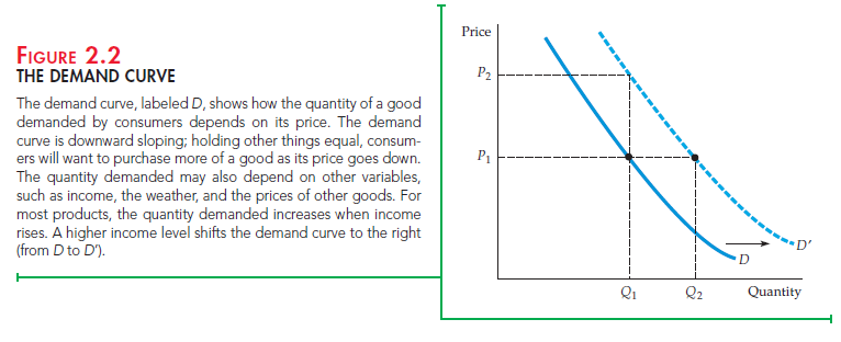
SHIFTING THE DEMAND CURVE Let’s see what happens to the demand curve if income levels increase. As you can see in Figure 2.2, if the market price were held constant at P1, we would expect to see an increase in the quan- tity demanded—say, from Q1 to Q2, as a result of consumers’ higher incomes. Because this increase would occur no matter what the market price, the result would be a shift to the right of the entire demand curve. In the figure, this is shown as a shift from D to D’. Alternatively, we can ask what price consumers would pay to purchase a given quantity Q1. With greater income, they should be will- ing to pay a higher price—say, P2 instead of P1 in Figure 2.2. Again, the demand curve will shift to the right. As we did with supply, we will use the phrase change in demand to refer to shifts in the demand curve, and reserve the phrase change in the quantity demanded to apply to movements along the demand curve.1
SUBSTITUTE AND COMPLEMENTARY GOODS Changes in the prices of related goods also affect demand. Goods are substitutes when an increase in the price of one leads to an increase in the quantity demanded of the other. For example, copper and aluminum are substitute goods. Because one can often be substituted for the other in industrial use, the quantity of copper demanded will increase if the price of aluminum increases. Likewise, beef and chicken are substi- tute goods because most consumers are willing to shift their purchases from one to the other when prices change.
Goods are complements when an increase in the price of one leads to a decrease in the quantity demanded of the other. For example, automobiles and gasoline are complementary goods. Because they tend to be used together, a decrease in the price of gasoline increases the quantity demanded for automobiles. Likewise, computers and computer software are complementary goods. The price of com- puters has dropped dramatically over the past decade, fueling an increase not only in purchases of computers, but also purchases of software packages.
We attributed the shift to the right of the demand curve in Figure 2.2 to an increase in income. However, this shift could also have resulted from either an increase in the price of a substitute good or a decrease in the price of a complementary good. Or it might have resulted from a change in some other variable, such as the weather. For example, demand curves for skis and snow- boards will shift to the right when there are heavy snowfalls.
Source: Pindyck Robert, Rubinfeld Daniel (2012), Microeconomics, Pearson, 8th edition.
The post Supply and Demand appeared first on HKT Consultant.
]]>The post The Market Mechanism appeared first on HKT Consultant.
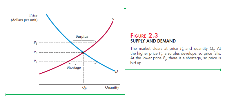
]]>EQUILIBRIUM The two curves intersect at the equilibrium, or market-clear- ing, price and quantity. At this price (P0 in Figure 2.3), the quantity supplied and the quantity demanded are just equal (to Q0). The market mechanism is the tendency in a free market for the price to change until the market clears— i.e., until the quantity supplied and the quantity demanded are equal. At this point, because there is neither excess demand nor excess supply, there is no pressure for the price to change further. Supply and demand might not always be in equilibrium, and some markets might not clear quickly when conditions change suddenly. The tendency, however, is for markets to clear.
To understand why markets tend to clear, suppose the price were initially above the market-clearing level—say, P1 in Figure 2.3. Producers will try to pro- duce and sell more than consumers are willing to buy. A surplus—a situation in which the quantity supplied exceeds the quantity demanded—will result. To sell this surplus—or at least to prevent it from growing—producers would begin to lower prices. Eventually, as price fell, quantity demanded wouldincrease, and quantity supplied would decrease until the equilibrium price P0 was reached.
The opposite would happen if the price were initially below P0—say, at P2. A shortage—a situation in which the quantity demanded exceeds the quantity supplied—would develop, and consumers would be unable to purchase all they would like. This would put upward pressure on price as consumers tried to outbid one another for existing supplies and producers reacted by increasing price and expanding output. Again, the price would eventually reach P0.
WHEN CAN WE USE THE SUPPLY-DEMAND MODEL? When we draw and use supply and demand curves, we are assuming that at any given price, a given quantity will be produced and sold. This assumption makes sense only if a market is at least roughly competitive. By this we mean that both sellers and buyers should have little market power—i.e., little ability individually to affect the market price.
Suppose instead that supply were controlled by a single producer—a monop- olist. In this case, there will no longer be a simple one-to-one relationship between price and the quantity supplied. Why? Because a monopolist’s behav- ior depends on the shape and position of the demand curve. If the demand curve shifts in a particular way, it may be in the monopolist’s interest to keep the quantity fixed but change the price, or to keep the price fixed and change the quantity. (How this could occur is explained in Chapter 10.) Thus when we work with supply and demand curves, we implicitly assume that we are refer- ring to a competitive market.
Source: Pindyck Robert, Rubinfeld Daniel (2012), Microeconomics, Pearson, 8th edition.
The post The Market Mechanism appeared first on HKT Consultant.
]]>The post Changes in Market Equilibrium appeared first on HKT Consultant.
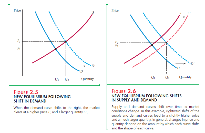
]]>Let’s begin with a shift in the supply curve. In Figure 2.4, the supply curve has shifted from S to S’ (as it did in Figure 2.1), perhaps as a result of a decrease in the price of raw materials. As a result, the market price drops (from P1 to P3), and the total quantity produced increases (from Q1 to Q3). This is what we would expect: Lower costs result in lower prices and increased sales. (Indeed, gradual decreases in costs resulting from technological progress and better management are an important driving force behind economic growth.)
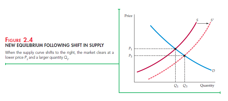
Figure 2.5 shows what happens following a rightward shift in the demand curve resulting from, say, an increase in income. A new price and quan- tity result after demand comes into equilibrium with supply. As shown in Figure 2.5, we would expect to see consumers pay a higher price, P3, and firms produce a greater quantity, Q3, as a result of an increase in income.
In most markets, both the demand and supply curves shift from time to time. Consumers’ disposable incomes change as the economy grows (or con-tracts, during economic recessions). The demands for some goods shift with the seasons (e.g., fuels, bathing suits, umbrellas), with changes in the prices of related goods (an increase in oil prices increases the demand for natural gas), or simply with changing tastes. Similarly, wage rates, capital costs, and the prices of raw materials also change from time to time, and these changes shift the supply curve.
Supply and demand curves can be used to trace the effects of these changes.
In Figure 2.6, for example, shifts to the right of both supply and demand result in a slightly higher price (from P1 to P2) and a much larger quantity (from Q1 to Q2). In general, price and quantity will change depending both on how much the supply and demand curves shift and on the shapes of those curves. To predict the sizes and directions of such changes, we must be able to character- ize quantitatively the dependence of supply and demand on price and other variables. We will turn to this task in the next section.
The post Changes in Market Equilibrium appeared first on HKT Consultant.
]]>The post Elasticities of Supply and Demand appeared first on HKT Consultant.
]]>We have seen that the demand for a good depends not only on its price, but also on consumer income and on the prices of other goods. Likewise, supply depends both on price and on variables that affect production cost. For example, if the price of coffee increases, the quantity demanded will fall and the quantity supplied will rise. Often, however, we want to know how much the quantity sup- plied or demanded will rise or fall. How sensitive is the demand for coffee to its price? If price increases by 10 percent, how much will the quantity demanded change? How much will it change if income rises by 5 percent? We use elasticities to answer questions like these.
An elasticity measures the sensitivity of one variable to another. Specifically, it is a number that tells us the percentage change that will occur in one variable in response to a 1-percent increase in another variable. For example, the price elasticity of demand measures the sensitivity of quantity demanded to price changes. It tells us what the percentage change in the quantity demanded for a good will be fol- lowing a 1-percent increase in the price of that good.
PRICE ELASTICITY OF DEMAND Let’s look at this in more detail. We write the price elasticity of demand, Ep, as

where % AQ means “percentage change in quantity demanded” and %AP means “percentage change in price.” (The symbol A is the Greek capital letter delta; it means “the change in.” So AX means “the change in the variable X,” say, from one year to the next.) The percentage change in a variable is just the absolute change in the variable divided by the original level of the variable. (If the Consumer Price Index were 200 at the beginning of the year and increased to 204 by the end of the year, the percentage change—or annual rate of inflation—would be 4/200 = .02, or 2 percent.) Thus we can also write the price elasticity of demand as follows:[1]
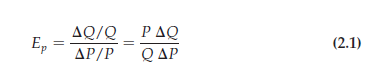
The price elasticity of demand is usually a negative number. When the price of a good increases, the quantity demanded usually falls. Thus AQ/ AP (the change in quantity for a change in price) is negative, as is E . Sometimes we refer to the magnitude of the price elasticity—i.e., its absolute size. For example, if Ep = – 2, we say that the elasticity is 2 in magnitude.
When the price elasticity is greater than 1 in magnitude, we say that demand is price elastic because the percentage decline in quantity demanded is greater than the percentage increase in price. If the price elasticity is less than 1 in magnitude, demand is said to be price inelastic. In general, the price elasticity of demand for a good depends on the availability of other goods that can be substituted for it. When there are close substitutes, a price increase will cause the consumer to buy less of the good and more of the substitute. Demand will then be highly price elastic. When there are no close substitutes, demand will tend to be price inelastic.
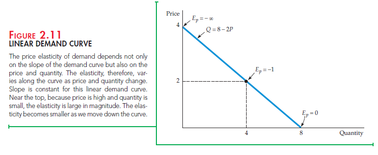
LINEAR DEMAND CURVE Equation (2.1) says that the price elasticity of demand is the change in quantity associated with a change in price (A Q/ A P) times the ratio of price to quantity (P/Q). But as we move down the demand curve, AQ/APmay change, and the price and quantity will always change. Therefore, the price elasticity of demand must be measured at a particular point on the demand curve and will generally change as we move along the curve.
This principle is easiest to see for a linear demand curve—that is, a demand curve of the form
Q = a – bP
As an example, consider the demand curve
Q = 8 – 2P
For this curve, AQ/AP is constant and equal to — 2 (a AP of 1 results in a AQ of —2). However, the curve does not have a constant elasticity. Observe from Figure 2.11 that as we move down the curve, the ratio P/Q falls; the elasticity therefore decreases in magnitude. Near the intersection of the curve with the price axis, Q is very small, so Ep = — 2(P/Q) is large in magnitude. When P = 2 and Q = 4 , Ep = — 1. At the intersection with the quantity axis, P = 0 so EP = 0.
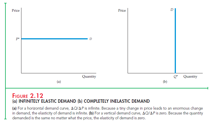
Because we draw demand (and supply) curves with price on the vertical axis and quantity on the horizontal axis, AQ/AP = (1/slope of curve). As a result, for any price and quantity combination, the steeper the slope of the curve, the less elastic is demand. Figure 2.12 shows two special cases. Figure 2.12(a) shows a demand curve reflecting infinitely elastic demand: Consumers will buy as much as they can at a single price P*. For even the smallest increase in price above this level, quantity demanded drops to zero, and for any decrease in price, quantity demanded increases without limit. The demand curve in Figure 2.12(b), on the other hand, reflects completely inelastic demand: Consumers will buy a fixed quantity Q*, no matter what the price.
OTHER DEMAND ELASTICITIES We will also be interested in elasticities of demand with respect to other variables besides price. For example, demand for most goods usually rises when aggregate income rises. The income elasticity of demand is the percentage change in the quantity demanded, Q, resulting from a 1-percent increase in income I:

The demand for some goods is also affected by the prices of other goods. For example, because butter and margarine can easily be substituted for each other, the demand for each depends on the price of the other. A cross-price elasticity of demand refers to the percentage change in the quantity demanded for a good that results from a 1-percent increase in the price of another good. So the elasticity of demand for butter with respect to the price of margarine would be written as
The demand for some goods is also affected by the prices of other goods. For example, because butter and margarine can easily be substituted for each other, the demand for each depends on the price of the other. A cross-price elasticity of demand refers to the percentage change in the quantity demanded for a good that results from a 1-percent increase in the price of another good. So the elasticity of demand for butter with respect to the price of margarine would be written as where Qb is the quantity of butter and Pm is the price of margarine.
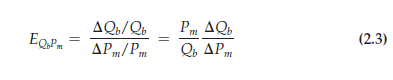
gasoline demanded falls—motorists will drive less. And because people are driving less, the demand for motor oil also falls. (The entire demand curve for motor oil shifts to the left.) Thus, the cross-price elasticity of motor oil with respect to gasoline is negative.
ELASTICITIES OF SUPPLY Elasticities of supply are defined in a similar manner. The price elasticity of supply is the percentage change in the quantity supplied resulting from a 1-percent increase in price. This elasticity is usually positive because a higher price gives producers an incentive to increase output.
We can also refer to elasticities of supply with respect to such variables as interest rates, wage rates, and the prices of raw materials and other intermediate goods used to manufacture the product in question. For example, for most manufactured goods, the elasticities of supply with respect to the prices of raw materials are negative. An increase in the price of a raw material input means higher costs for the firm; other things being equal, therefore, the quantity supplied will fall.
Point versus Arc Elasticities
So far, we have considered elasticities at a particular point on the demand curve or the supply curve. These are called point elasticities. The point elasticity of demand, for example, is the price elasticity of demand at a particular point on the demand curve and is defined by Equation (2.1). As we demonstrated in Figure 2.11 using a linear demand curve, the point elasticity of demand can vary depending on where it is measured along the demand curve.
There are times, however, when we want to calculate a price elasticity over some portion of the demand curve (or supply curve) rather than at a single point. Suppose, for example, that we are contemplating an increase in the price of a product from $8.00 to $10.00 and expect the quantity demanded to fall from 6 units to 4. How should we calculate the price elasticity of demand? Is the price increase 25 percent (a $2 increase divided by the original price of $8), or is it 20 percent (a $2 increase divided by the new price of $10)? Is the percentage decrease in quantity demanded 33 1/3 percent (2/6) or 50 percent (2/4)?
There is no correct answer to such questions. We could calculate the price elasticity using the original price and quantity. If so, we would find that Ep = (- 33 1/3 percent/25 percent) = -1.33. Or we could use the new price and quantity, in which case we would find that Ep = (- 50 percent/20 percent) = – 2.5. The difference between these two calculated elastici ties is large, and neither seems preferable to the other.
ARC ELASTICITY OF DEMAND We can resolve this problem by using the arc elasticity of demand: the elasticity calculated over a range of prices. Rather than choose either the initial or the final price, we use an average of the two, P; for the quantity demanded, we use Q. Thus the arc elasticity of demand is given by Arc elasticity: 
In our example, the average price is $9 and the average quantity 5 units. Thus the arc elasticity is
Ep = ( – 2/$2)($9/5) = -1.8
The arc elasticity will always lie somewhere (but not necessarily halfway) between the point elasticities calculated at the lower and the higher prices.
Although the arc elasticity of demand is sometimes useful, economists generally use the word “elasticity” to refer to a point elasticity. Throughout the rest of this book, we will do the same, unless noted otherwise.
Source: Pindyck Robert, Rubinfeld Daniel (2012), Microeconomics, Pearson, 8th edition.
The post Elasticities of Supply and Demand appeared first on HKT Consultant.
]]>The post Short-Run versus Long-Run Elasticities appeared first on HKT Consultant.
]]>1. Demand
For many goods, demand is much more price elastic in the long run than in the short run. For one thing, it takes time for people to change their consump- tion habits. For example, even if the price of coffee rises sharply, the quantity demanded will fall only gradually as consumers begin to drink less. In addi- tion, the demand for a good might be linked to the stock of another good that changes only slowly. For example, the demand for gasoline is much more elastic in the long run than in the short run. A sharply higher price of gaso- line reduces the quantity demanded in the short run by causing motorists to drive less, but it has its greatest impact on demand by inducing consum- ers to buy smaller and more fuel-efficient cars. But because the stock of cars changes only slowly, the quantity of gasoline demanded falls only slowly. Figure 2.13(a) shows short-run and long-run demand curves for goods such as these.
DEMAND AND DURABILITY On the other hand, for some goods just the opposite is true—demand is more elastic in the short run than in the long run. Because these goods (automobiles, refrigerators, televisions, or the capital equip- ment purchased by industry) are durable, the total stock of each good owned by consumers is large relative to annual production. As a result, a small change in the total stock that consumers want to hold can result in a large percentage change in the level of purchases.
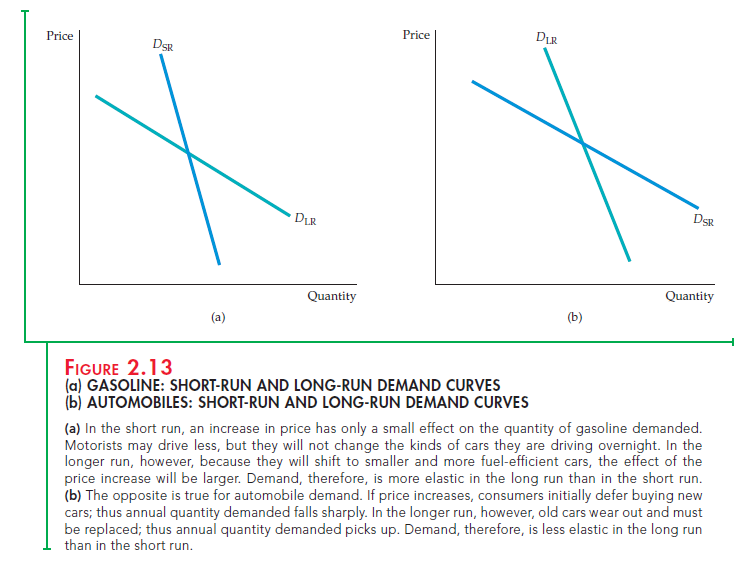
Suppose, for example, that the price of refrigerators goes up 10 percent, caus- ing the total stock of refrigerators that consumers want to hold to drop 5 percent. Initially, this will cause purchases of new refrigerators to drop much more than
5 percent. But eventually, as consumers’ refrigerators depreciate (and units must be replaced), the quantity demanded will increase again. In the long run, the total stock of refrigerators owned by consumers will be about 5 percent less than before the price increase. In this case, while the long-run price elasticity of demand for refrigerators would be – .05/.10 = – 0.5, the short-run elasticity would be much larger in magnitude.
Or consider automobiles. Although annual U.S. demand—new car pur- chases—is about 10 to 12 million, the stock of cars that people own is around
130 million. If automobile prices rise, many people will delay buying new cars. The quantity demanded will fall sharply, even though the total stock of cars that consumers might want to own at these higher prices falls only a small amount. Eventually, however, because old cars wear out and must be replaced, the quantity of new cars demanded picks up again. As a result, the long-run change in the quantity demanded is much smaller than the short- run change. Figure 2.13(b) shows demand curves for a durable good like automobiles.
INCOME ELASTICITIES Income elasticities also differ from the short run to the long run. For most goods and services—foods, beverages, fuel, entertain- ment, etc.—the income elasticity of demand is larger in the long run than in the short run. Consider the behavior of gasoline consumption during a period of strong economic growth during which aggregate income rises by
10 percent. Eventually people will increase gasoline consumption because they can afford to take more trips and perhaps own larger cars. But this change in consumption takes time, and demand initially increases only by a small amount. Thus, the long-run elasticity will be larger than the short-run elasticity.
For a durable good, the opposite is true. Again, consider automobiles. If aggregate income rises by 10 percent, the total stock of cars that consumers will want to own will also rise—say, by 5 percent. But this change means a much larger increase in current purchases of cars. (If the stock is 130 million, a 5-percent increase is 6.5 million, which might be about 60 to 70 percent of normal demand in a single year.) Eventually consumers succeed in increasing the total number of cars owned; after the stock has been rebuilt, new purchases are made largely to replace old cars. (These new purchases will still be greater than before because a larger stock of cars outstanding means that more cars need to be replaced each year.) Clearly, the short-run income elasticity of demand will be much larger than the long-run elasticity.
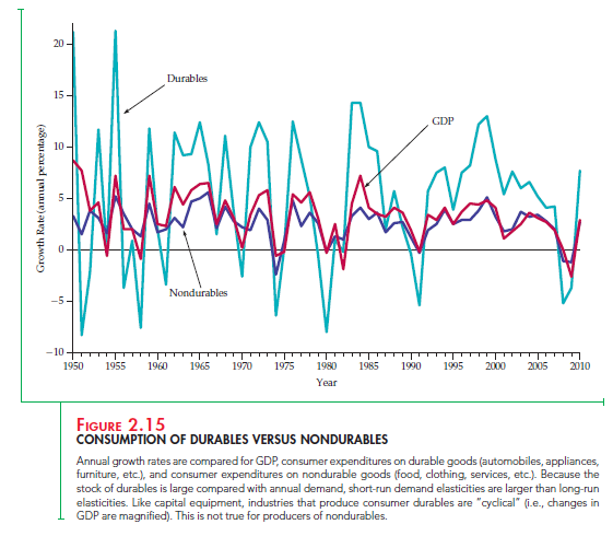
CYCLICAL INDUSTRIES Because the demands for durable goods fluctuate so sharply in response to short-run changes in income, the industries that produce these goods are quite vulnerable to changing macroeconomic condi- tions, and in particular to the business cycle—recessions and booms. Thus, these industries are often called cyclical industries—their sales patterns tend to magnify cyclical changes in gross domestic product (GDP) and national income.
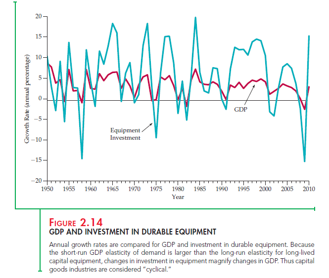
Figures 2.14 and 2.15 illustrate this principle. Figure 2.14 plots two variables over time: the annual real (inflation-adjusted) rate of growth of GDP and the annual real rate of growth of investment in producers’ durable equipment (i.e., machinery and other equipment purchased by firms). Note that although the durable equipment series follows the same pattern as the GDP series, the changes in GDP are magnified. For example, in 1961–1966 GDP grew by at least
4 percent each year. Purchases of durable equipment also grew, but by much more (over 10 percent in 1963–1966). Equipment investment likewise grew much more quickly than GDP during 1993–1998. On the other hand, during the recessions of 1974–1975, 1982, 1991, 2001, and 2008, equipment purchases fell by much more than GDP.
Figure 2.15 also shows the real rate of growth of GDP, along with the annual real rates of growth of spending by consumers on durable goods (automobiles, appliances, etc.) and nondurable goods (food, fuel, clothing, etc.). Note that while both consumption series follow GDP, only the durable goods series tends to magnify changes in GDP. Changes in consumption of nondurables are roughly the same as changes in GDP, but changes in con- sumption of durables are usually several times larger. This is why companies such as General Motors and General Electric are considered “cyclical”: Sales of cars and electrical appliances are strongly affected by changing macroeco- nomic conditions.
2. Supply
Elasticities of supply also differ from the long run to the short run. For most products, long-run supply is much more price elastic than short-run supply: Firms face capacity constraints in the short run and need time to expand capacity by building new production facilities and hiring workers to staff them. This is not to say that the quantity supplied will not increase in the short run if price goes up sharply. Even in the short run, firms can increase output by using their existing facilities for more hours per week, paying workers to work overtime, and hiring some new workers immediately. But firms will be able to expand output much more when they have the time to expand their facilities and hire larger permanent workforces.
For some goods and services, short-run supply is completely inelastic. Rental housing in most cities is an example. In the very short run, there is only a fixed number of rental units. Thus an increase in demand only pushes rents up. In the longer run, and without rent controls, higher rents provide an incentive to renovate existing buildings and construct new ones. As a result, the quantity supplied increases.
For most goods, however, firms can find ways to increase output even in the short run—if the price incentive is strong enough. However, because various constraints make it costly to increase output rapidly, it may require large price increases to elicit small short-run increases in the quantity supplied. We discuss these characteristics of supply in more detail in Chapter 8.
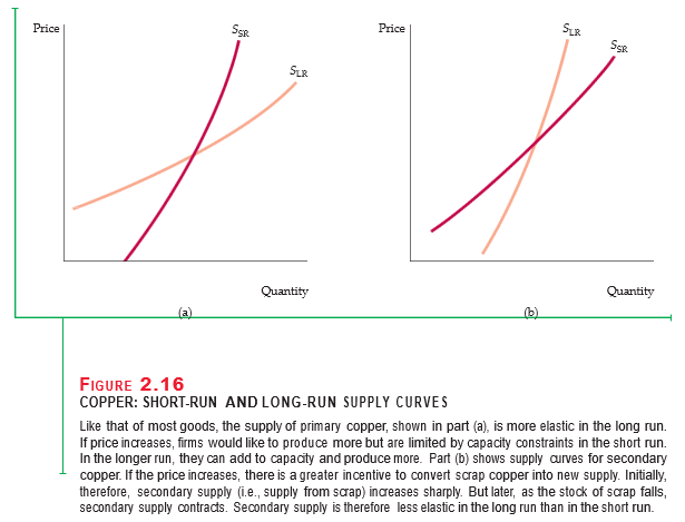
SUPPLY AND DURABILITY For some goods, supply is more elastic in the short run than in the long run. Such goods are durable and can be recycled as part of supply if price goes up. An example is the secondary supply of metals: the supply from scrap metal, which is often melted down and refabricated. When the price of copper goes up, it increases the incentive to convert scrap copper into new supply, so that, initially, secondary supply increases sharply. Eventually, how- ever, the stock of good-quality scrap falls, making the melting, purifying, and refabricating more costly. Secondary supply then contracts. Thus the long-run price elasticity of secondary supply is smaller than the short-run elasticity.
Figures 2.16(a) and 2.16(b) show short-run and long-run supply curves for primary (production from the mining and smelting of ore) and secondary copper production. Table 2.3 shows estimates of the elasticities for each component of supply and for total supply, based on a weighted average of the component elasticities.12 Because secondary supply is only about 20 percent of total supply, the price elasticity of total supply is larger in the long run than in the short run.
Source: Pindyck Robert, Rubinfeld Daniel (2012), Microeconomics, Pearson, 8th edition.
The post Short-Run versus Long-Run Elasticities appeared first on HKT Consultant.
]]>