The post Introduction to Eviews appeared first on HKT Consultant.
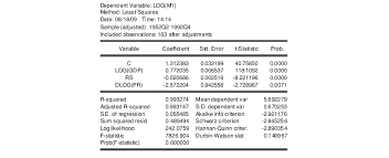
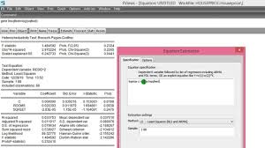
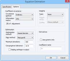
]]>EViews is a software package that provides tools for data analysis, regression, and forecasting. It is a “canned” regression package for econometric analysis. EViews has an object-oriented design. Each type of object has specific ‘views’ and procedures that are used in Eviews.
Eviews has been a command-line-only program up until recently, and all the advanced features, such as Kronecker products, eigenvector solution, and singular value decomposition are still processed using the command line. As well, the command line mode records all of the steps in an analysis. The GUI (Graphical User Interface) is convenient, but you will have no record of your session and will have to go back to command line mode to use advanced features.
Main contentsSee more from basic to advanced
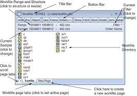
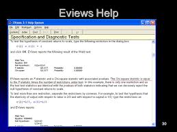

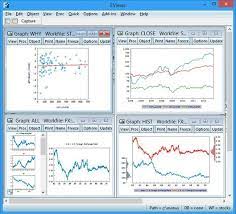


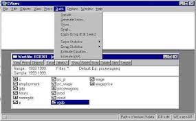
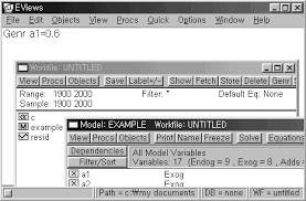
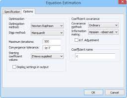
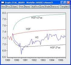

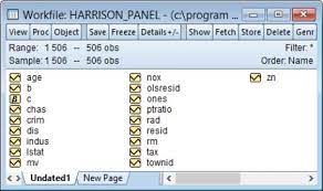
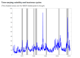

The post Introduction to Eviews appeared first on HKT Consultant.
]]>The post Using EViews for Principles of Econometrics appeared first on HKT Consultant.
]]>1. Installing EViews 6 student version
Your copy of EViews is distributed on a single CD-ROM. EViews is a Windows-based program. First close all other applications, then insert the CD into your computer’s drive and wait until the setup program launches. If the CD does not spin-up on its own, navigate to the CD drive using Windows Explorer, and click on the Setup icon (AUTORUN.EXE).
The initial screen is shown below. You should first click on View Read Me to see any last minute changes or instructions. Click View Documentation to open EViews 6 Getting Started for the Student Version. It describes the installation and registration process. This document can also be accessed from the Help/Student Version Getting Started (pdf) from the main EViews menu. You must have Adobe Acrobat to read *.pdf files. If you do not have this software, go to www.adobe.com and download the free Adobe Reader.
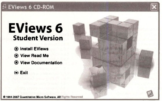
When you are ready, click Install EViews and follow the on-screen instructions.
2. Checking for updates
Once installed you should visit www.eviews.com and check the “download” link. There you will find any updates for your software.
3. Obtaining data workfiles
The EViews data workfiles (with extension *.wfl) and other resources for POE can be found at www.wilev.com/college/hill . Find the link “Online resources for students.” The POE workfiles can be downloaded in a compressed format, saved to a subdirectory (we use c:\data\eviews), and then expanded. In addition to the EViews workfiles, there are “data definition” files (*.def) that describe the variables and show some summary statistics. The definition files are simple text files that can be opened with utilities like Notepad or Wordpad, or using a word processor. These files should be downloaded as well. Individual EViews workfiles, definition files, and other resources can be obtained at www.bus.lsu.edu/hill/poe. The data files in EViews, Excel, and ASCII format, along with the definition files, are also on the EViews 6 SV CD-ROM that came with this manual.
Main contentsSee more from basic to advanced
Source: Griffiths William E., Hill R. Carter, Lim Mark Andrew (2008), Using EViews for Principles of Econometrics, John Wiley & Sons; 3rd Edition.
The post Using EViews for Principles of Econometrics appeared first on HKT Consultant.
]]>The post Starting EViews appeared first on HKT Consultant.
]]>
Alternatively, select EViews from the Windows Start Menu. When EViews opens you are presented with the following screen

Across the top are Drop Down Menus that make implementing EViews procedures quite simple. Below the menu items is the Command Line. It can be used as an alternative to the menus, once you become familiar with basic commands and syntax. Across the bottom is the Current Path for reading data and saving files. The EViews Help Menu is going to become a close friend.
Source: Griffiths William E., Hill R. Carter, Lim Mark Andrew (2008), Using EViews for Principles of Econometrics, John Wiley & Sons; 3rd Edition.
The post Starting EViews appeared first on HKT Consultant.
]]>The post The EViews Help System appeared first on HKT Consultant.
]]>
The resulting menu is

1. EViews help topics
First, click on EViews Help Topics. Select Getting Started (Student Version) to obtain basic information about the Student Version of EViews. Selecting User’s Guide/EViews Fundamentals opens a list of chapters that can take you through specifics of working with EViews. These guides will be a useful reference after you have progressed further through Using EViews for POE.

2. The read me file
On the Help menu, select READ ME. This opens a PDF file with the latest installation notes and errata.

3. Quick help reference
Select Quick Help Reference. You find another menu. Select Function Reference.

EViews has many, many functions available for easy use.
- Operato
- Basie mathematical functions.
- Time series functions.
- Financial functions.
- Descriptive statistics.
- Cumulative statistics functions.
- Moving statistics functions.
- Group row functions.
- By-group statistics.
- Additional and special functions.
- Trigonometric functions.
- Statisncai oistridution functions.
You should just take a moment to examine the Operators (basic addition, multiplication, etc.) and the Basic mathematical functions (square roots, logarithms, absolute value, etc.). This Function Reference help is one that you will use very frequently, and to which we will refer a great deal.
4. EViews Illustrated
The next Help menu item is for sample chapters from EViews Illustrated by Richard Startz, which is good humored tutorial, with screen shots like you are seeing here, covering many aspects of using EViews. The first three chapters are provided.

5. Users Guides and Command Reference
The User’s Guide I (794 pages), User’s Guide II (688 pages) and Command Reference (926 pages) are the complete documentation for the full version of EViews 6. While these are good rainy day reading we do not necessarily suggest you search them for information until you are more familiar with the workings of EViews. This book, Using EViews for POE, is an effort to guide you through the essentials of EViews that are needed to replicate the examples in the book POE.
Source: Griffiths William E., Hill R. Carter, Lim Mark Andrew (2008), Using EViews for Principles of Econometrics, John Wiley & Sons; 3rd Edition.
The post The EViews Help System appeared first on HKT Consultant.
]]>The post Using a EViews Workfile appeared first on HKT Consultant.
]]>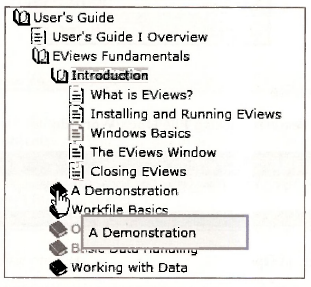
The demonstration starts by importing data into EViews from an Excel spreadsheet. We will skip that step here, but if you like you can gain further practice by following along their demonstration.
Remark: You will want to be able to “import” data into EViews, or enter data manually. We cover the various methods for entering data into EViews in Chapter 17 of this manual.
1. Setting the default path
At the bottom of the EViews screen you will see Path = . This determines where EViews will first look for data and save workfiles.

Double-click on Path and a window will open in which you can locate what you desire for your default directory. We will use the path c:\data\eviews
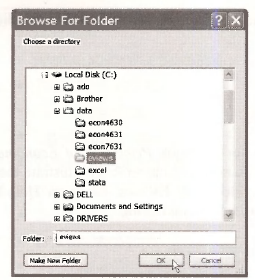
2. Opening a workfile
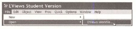
Open the workfile called demo by clicking File/Open/Workfile
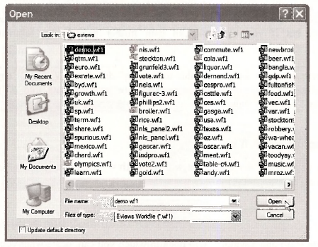
Select demo.wfl and click on Open.
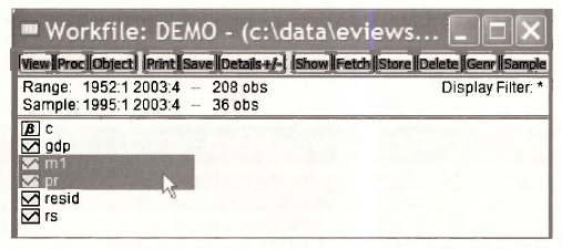
The workfile opens to show
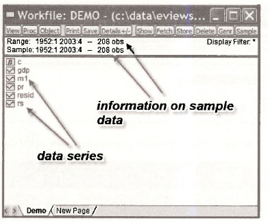
Located on the left side are data series that are indicated by the icon 0. EViews calls the elements of the workfile objects. As you will discover, there are many types of objects that EViews can save into the workfile—not only series but tables, graphs, equations, and so on. As Richard Startz says, an object is a little “thingie” that computer programmers talk about. Each little icon “thingie” in the workfile is an object.
In this workfile the data series, or variables, are:
- GDP—gross domestic product
- Ml—money supply
- PR—price level (index)
- RS—short term interest rate
The series resid and the icon labeled p are always present in EViews workfiles (even new ones with no data) and their use will be explained later. Across the top of the workfile are various buttons that initiate tasks in EViews, and these too will be explained later.
Below the buttons are Range: 1952:1 2003:4, which indicates that the 208 observations on the variables included run from 1952, Quarter 1, to 2003, Quarter 4. Sample: 1952:1 2003:4 denotes the data observations EViews will use in calculations. Many times we will choose for analysis less than the full range of observations that are available, so Sample will differ from Range.
3. Examing a single series
It is a good idea each time you open a workfile to look at one or more series just to verify that the data are what you expect. First, select one series
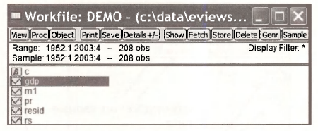
Double-click in the blue area, which will reveal a spreadsheet view of the data.
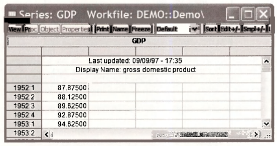
In the upper left hand corner is a button labeled View

This opens a drop-down menu with a number of choices. Select Descriptive Statistics & Tests/Histogram and Stats.
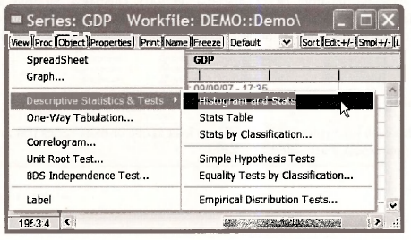
The result is
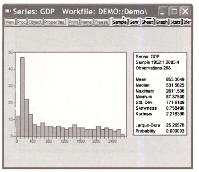
This histogram is shown with various summary statistics on the side. Click on View again. Select Graph.
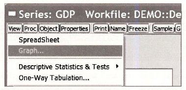
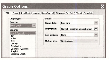
There you will see many options. The default graph type is a Basic Graph with the Line & Symbol plotted. Select OK.
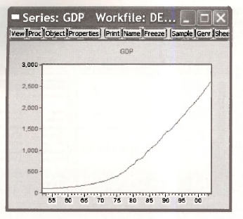
The result is a line graph. The dates are on the horizontal axis and GDP on the vertical axis.
4. Changing the sample
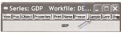
If you wish to view the graph or summary statistics for a different sample period, click on the Sample button. This feature works the same in all EViews windows.
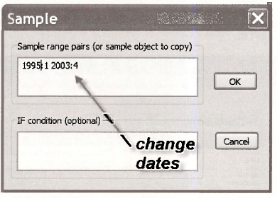
In the dialog box that opens change the sample to 1995:1 to 2003:4 then click OK.
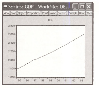
The resulting graph shows that GDP rose constantly during this period.
5. Copying graph into a document
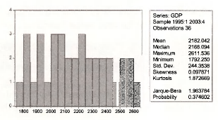
Select View/Descriptive Statistics & Tests/Histogram and Stats. You will find now the summary statistics and histogram of GDP for the period 1995:1 to 2003:4. These results can be printed by selecting the Print button.

You may prefer to copy the results into a word processor for later editing and combining results. How can results be taken from EViews into a document? Click inside the histogram
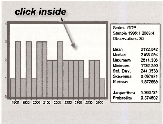
While holding down the Ctrl key press C (which we will denote as Ctrl+C). This is the Windows keystroke combination for Copy.
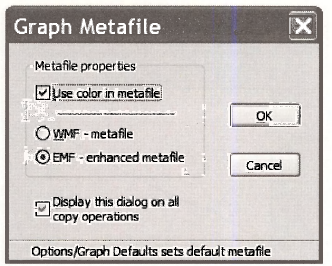
In the resulting dialog box you can make some choices, then click OK. This copies the graph into the Windows clipboard (memory). Open a document in your word processor and enter Ctrl+V which will Paste the figure into your document.
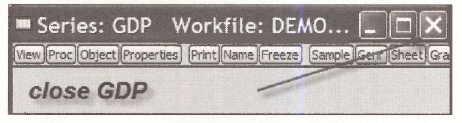
Lets close the graph we have been working on, by clicking the red X in the upper right hand comer of the GDP screen
Source: Griffiths William E., Hill R. Carter, Lim Mark Andrew (2008), Using EViews for Principles of Econometrics, John Wiley & Sons; 3rd Edition.
The post Using a EViews Workfile appeared first on HKT Consultant.
]]>The post Examining Several Series with EViews appeared first on HKT Consultant.
]]>
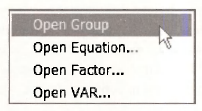
Click on Open Group.
A spreadsheet view of the data will open.
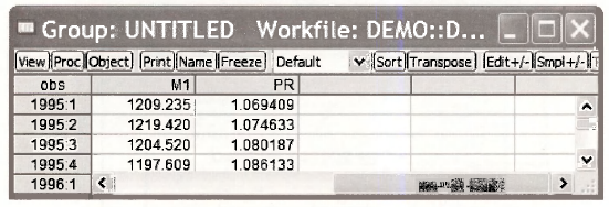
Note that the series begins in 1995:1 because we changed the Sample range in Section 1.4.4.
1. Summary statistics for several series
From the spreadsheet we can again examine the data by selecting the View button. Select Descriptive Stats/Common Sample.
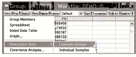
The result is a table of summary statistics is created for the two series (variables) in the group.
2. Freezing a result
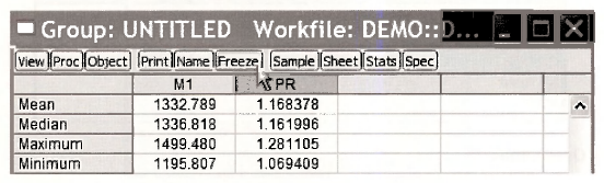
These results can be “saved” several ways. Select the Freeze button. This actually saves an image of the table. In the new image window, select the Name button. Enter a name for this image, which EViews calls an Object. The name should be relatively short and cannot contain any spaces. Often underscores can be used to separate words to make recognition easier.
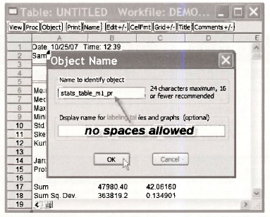
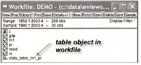
Click OK, then close the Object by clicking on the red X. Check back in the workfde and you will now see a new entry, which is the table you have created.
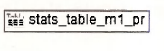
The table can be recalled at any time by double clicking the Table icon
3. Copying and pasting a table
To copy these into a document directly, highlight the table of results (drag the mouse while holding down its left button), enter Ctrl+C. In the resulting box click the Formatted radio button, check the box to Include header information, and click OK. This copies the table to the Windows clipboard, which then can be pasted (Ctrl+V) into an open document.
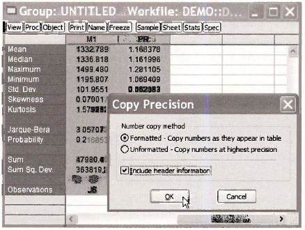
This same method can be used for basically any table in EViews. For example, if you open the saved table “STATS TABLE Ml PR” you can highlight the results, then copy and paste as we have done here.
4. Plotting two series
Return to the spreadsheet view of the two series Ml and PR. Select View/Graph. In the resulting dialog box, select Multiple graphs in the Multiple series menu.
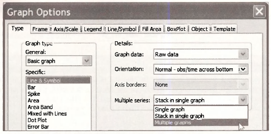
Click OK to obtain two plots of the series
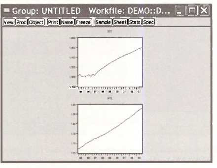
We can Freeze this picture, then assign it a Name for future reference.
5. A scatter diagram
A scatter diagram is a plot of the data points with one variable on one axis and the other variable on the other axis. In the Group screen click View/Graph. Select Scatter as the specific type of graph.
Click OK. Copy the graph by clicking inside the graph area, entering Ctrl+C to copy, then paste into a document using Ctrl+V. The resulting graph is on the next page. Recall that we are still operating with the sample from 1995:1 to 2003:4, which is only 36 data points.
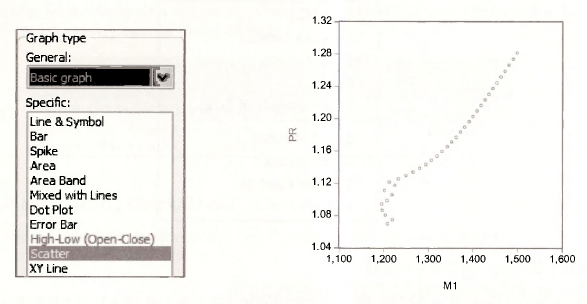
The variable Ml is on the horizontal axis because it is the first series in the spreadsheet view.
Click the red X in the Group window. When you do this you will be faced with some choices.
The Group consists of the two series Ml and PR. This Group can be saved by selecting Name and assigning a name.
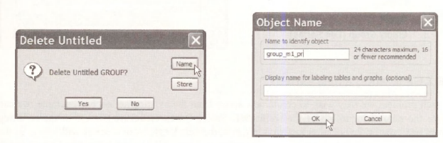
In the workfile window you will find a new object for this group.

Source: Griffiths William E., Hill R. Carter, Lim Mark Andrew (2008), Using EViews for Principles of Econometrics, John Wiley & Sons; 3rd Edition.
The post Examining Several Series with EViews appeared first on HKT Consultant.
]]>The post Using the Quick Menu of EViews appeared first on HKT Consultant.
]]>
The options shown are
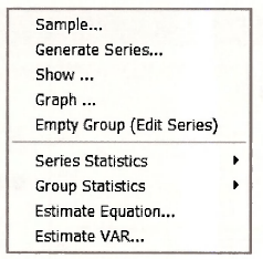
1. Changing the sample
By selecting Sample from this menu we can change the range of sample observations. Change the sample to 1952:1 to 2003:4 and click OK.
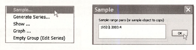
2. Generating a new series
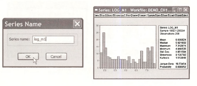
In each problem we may wish to create new series from the existing series. For example, we can create the natural logarithm of the series Ml. Select Quick/Generate Series. In the resulting dialog box type in the equation log_m1=log(m1), then click OK. A new series will appear in the workfde. The function log creates the natural logarithm. All logarithms use in Principles of Econometrics are natural logs.
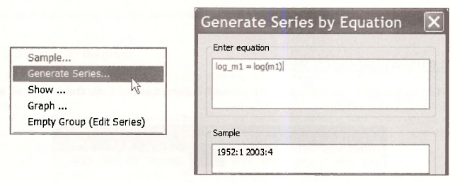
Alternatively, we can generate a new series by selecting the Genr button on the workfile menu. This will open the same Generate Series dialog box.
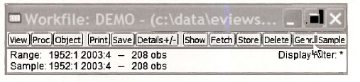
3. Plotting using Quick/Graph
We can create graphs from the spreadsheet view, but we can also use Quick/Graph.
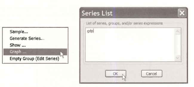
This will open the Graph options window. For a basic graph click OK.
If you enter two series into the Series List window then the Graph options window will have an additional option
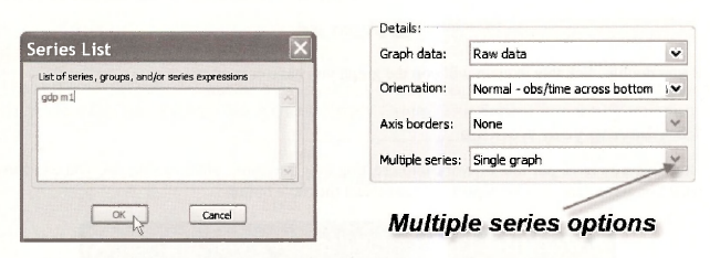
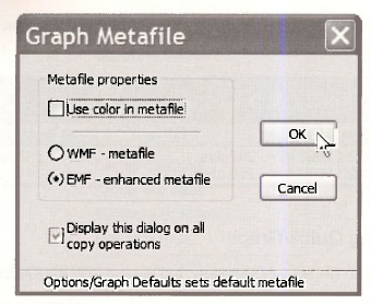
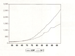
Click OK. The resulting graph shows the two series plots in a single window. In EViews the curves are in two different colors, but this will not show in a black and white document. The programmers at EViews have thought of this problem. Click inside the graph and enter Ctrl+C to copy. In the Graph Metafile box that opens uncheck the box “Use color in metafile.” Click OK.
In your document enter Ctrl+V to paste the black and white graph. Now the graph lines show up as solid for GDP and broken for Ml so that the difference can be viewed.
To save the graph, click Name and enter the name GDP_Ml_PLOT. Click OK. Close the graph by clicking “X”. You will find an icon in the workfile window.
If you double click this icon up will pop the graph you have created.
4. Saving your workfile
Now that you have put lots of work into creating new variables, plots, and so on, you can Save what you have done. On the workfile menu select the Save button
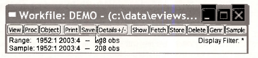
In the following window, IF you click OK then all the objects you have created will be saved into the workfile demo.wfl. You may wish to save these results using a different name, so that the original data workfile is not changed. To save the workfile, select File/Save As on the main EViews menu
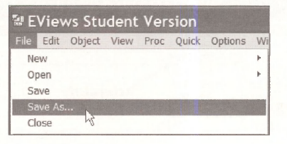
We will use the name demo chl.wfl for this workfile. Enter this and click OK. You will presented with some options. Use the default of Double precision and click OK.
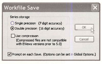
You will note that the workfile name has changed.
5. Opening an empty group
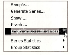
The ability to enter data manually is an important one. In Chapter 17 we show all the ways you might enter data into EViews. Select Quick/Empty Group (Edit Series) from the EViews menu.
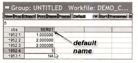
A spreadsheet opens into which you can enter new data. The default name for a new series is SER01 that we will change. As you enter a number press Enter to move to the next cell. You can add new data in as many columns as you like.
When you have finished entering the data you wish, click the red X in the upper right corner of the active window. You will be asked if you want to “Delete Untitled GROUP?” Select Yes. In the workfile demo chl.wfl you will now find the new series labeled

To change this name, select the series (by clicking) then right-click in the shaded area. A box will open in which you can enter a new name for the “object” which in this case is a data series. Press OK
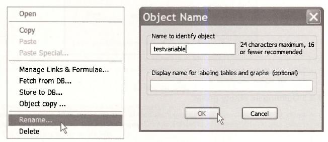
You can go through these same steps to delete an unwanted variable, such as the one we have just created. Select the series “TESTVARIABLE” in the workfile, and right click. Select Delete. In the resulting window you will be asked to confirm the deletion. Select Yes.

More than one series or objects can be selected for deletion by selecting one, then hold down the Ctrl-key while selecting others. To delete all these selected objects right-click in the blue area, and repeat the steps above.
6. Quick/Series statistics
The next item on the EViews Quick menu is Series Statistics. Select Quick/Series Statistics/Histogram and Stats

In the resulting window you can enter the name of the series (one) for a which you desire the summary statistics. Then select OK.
7. Quick/Group statistics
We can obtain summary statistics for a Group of series by choosing Quick/Group Statisitcs.
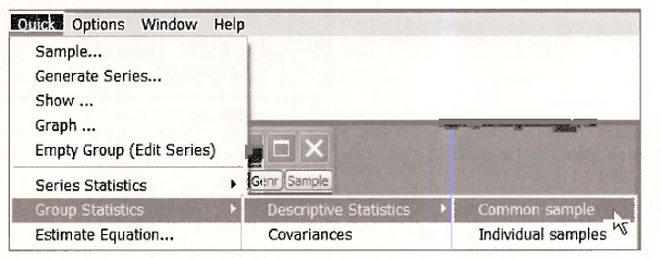
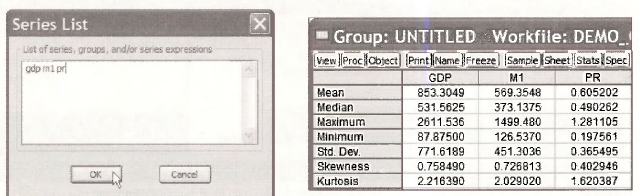
Enter the series names into the box and press OK. This will create the summary statistics table we have seen before. You can Name this group, or Freeze the table, or copy and paste using Ctrl+C and Ctrl+V.
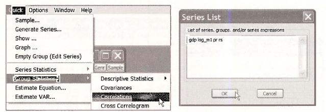
Another option under Quick/Group Statistics is Correlations. Enter the names of series for which the sample correlations are desired and click OK.
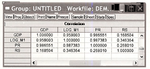
The sample correlations are arranged in an array, or matrix, format.
Source: Griffiths William E., Hill R. Carter, Lim Mark Andrew (2008), Using EViews for Principles of Econometrics, John Wiley & Sons; 3rd Edition.
The post Using the Quick Menu of EViews appeared first on HKT Consultant.
]]>The post Using EViews Functions appeared first on HKT Consultant.
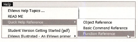
]]>
1. Descriptive statistics functions
Select Descriptive Statistics from the list of material links.
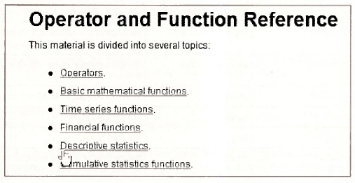
Some of the descriptive statistics functions listed there are on the next page.
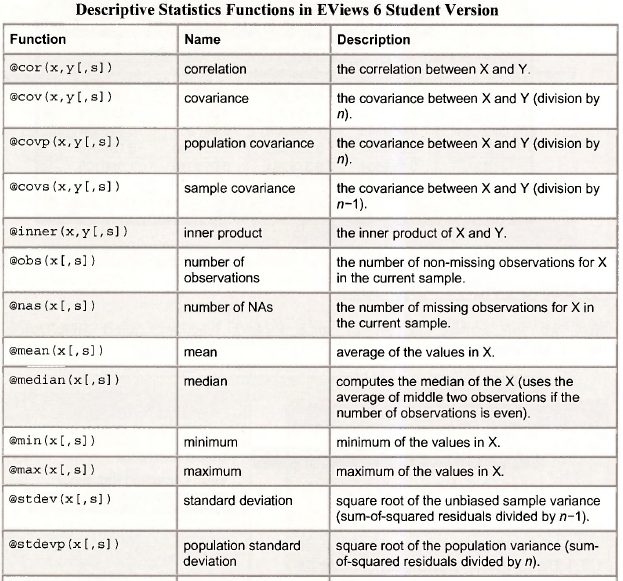
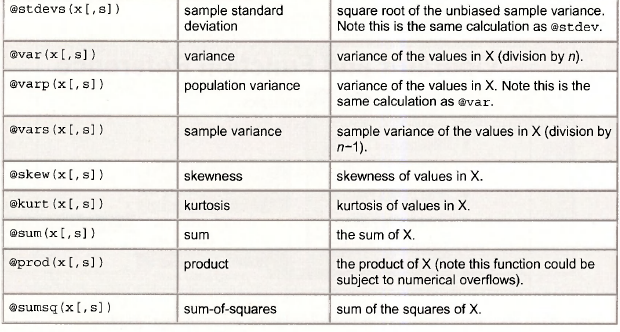
In this table of functions you will note that these functions begin with the (dr symbol. Also, these functions return a single number, which is called a scalar. In the commands the variables, or series, are called x and y. The bracket notation “[,s]” is optional and we will not use it. These functions are used by typing commands into the Command Window and pressing Enter. For example, to compute the sample mean of GDP type
scalar gdpbar = @mean(gdp).
The command window looks like this.

At the bottom of the EViews screen you will note the message

In the workfile window the new object is denote with “#” that indicates a scalar.

We called the sample mean GDPBAR because sample means are often denoted by symbols like x which is pronounced “x-bar.” In the “text messaging” world in which you live, simple but meaningful names will occur to you naturally.
To view this scalar object double click on it, or type show gdpbar in the Command window. At the bottom of the EViews screen you will see

The sample mean of GDP during the sample period is 853.305.
Scalars you have created can be used in further calculations. For example, enter the following commands by typing them into the command window and pressing Enter
scalar t = @obs(gdp)
scalar gdpse = @stdev(gdp)
scalar z = (gdpbar – 800)/(gdpse/@sqrt(t))
The value of z is 0.996, and is the test statistic value for the null hypothesis that the population mean of GDP equals 800. In the workfile are now objects for each of the scalars created.
2. Using a storage vector
The creation of scalars leads to inclusion of additional objects into the workfde, and the scalars cannot be viewed simultaneously. One solution is to create a storage vector into which these scalars can be placed.
On the EViews menu bar select Object/New Object. In the resulting dialog box select Matrix-Vector-Coef and enter an object name, say DEMO. Click OK.
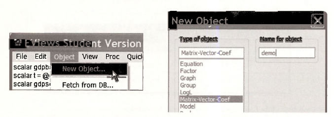
A dialog box will open asking what type of “new matrix” you want. To create a storage vector (an array) with 10 rows select the radio button Vector, enter 10 for Rows, and click OK.

A spreadsheet will open with rows labeled R1 to RIO. Now enter into the Command window the command
demo(1) = @mean(gdp)
When you press Enter the value in row R1 will change to 853.3049, the sample mean of GDP, as shown on the next page.
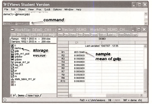
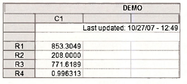
Now enter the series of commands, pressing Enter after each.
demo(2) = @obs(gdp)
demo(3) = @stdev(gdp)
demo(4) = (gdpbar – 800)/(gdpse/@sqrt(t))
Each time a command is entered a new item shows in the vector.
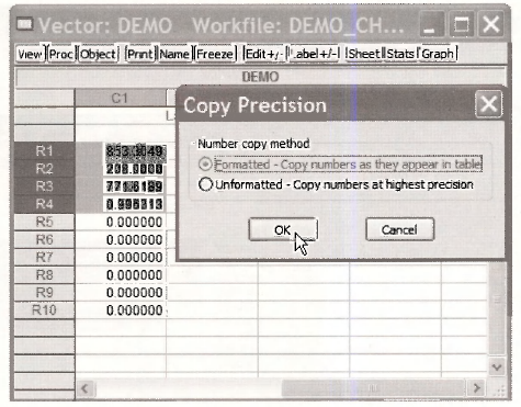
The advantage of this approach is that the contents of this table can be copied and pasted into a document for easy presentation. Highlight the contents, enter Ctrl+C. Choose the Formatted radio button and OK.
In an open document enter Ctrl+V to paste the table of results.
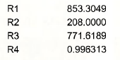
You can now edit as you would any table.
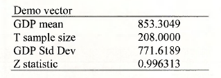
We created many tables in the book Principles of Econometrics using this method.
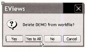
To keep our workfile tidy, delete the scalar and vector objects that have no further use. Click the vector object DEMO and then while holding down the Ctrl-key, click on the scalars. Right- click in the blue-shaded area and select Delete.
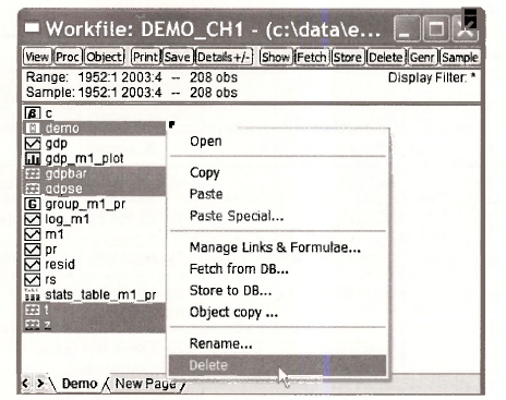
If you feel confident you can choose Yes to All
3. Basic arithmetic operations
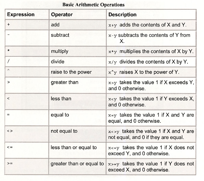
The basic arithmetic operations can be viewed at Help/Quick Help Reference/Function Reference
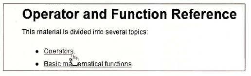
The list of operators is given on the next page. These operators can be used when working with series, such as in an operation to generate a new series, RATIOl, such as 3 times the ratio of GDP to Ml:
series ratiol = 3*(gdp/m1)
4. Basic math functions
The basic math functions can be viewed at Help/Quick Help Reference/Function Reference
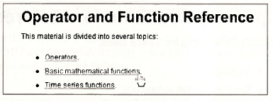
Some of these functions are listed below. Note that common ones like the absolute value (abs), the exponential function (exp), the natural logarithm (log) and the square root (sqr) can be used with or without the @ sign.

Source: Griffiths William E., Hill R. Carter, Lim Mark Andrew (2008), Using EViews for Principles of Econometrics, John Wiley & Sons; 3rd Edition.
The post Using EViews Functions appeared first on HKT Consultant.
]]>The post The Simple Linear Regression Model by using EViews appeared first on HKT Consultant.
]]>1. OPEN THE WORKFILE
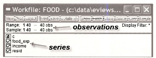
The data for the food expenditure example are contained in the workfile food.wfl. Locate this file and open it by selecting File/Open/EViews Workfile

The initial workfile contains two variables INCOME, which is weekly household income, and FOOD EXP, which is household weekly household food expenditure. See the definition file foocLdef for the variable definitions.
1.1. Examine the data
When ever opening a new workfile it is prudent to examine the data. Select INCOME by clicking it, and then while holding the Ctrl-key select FOOD EXP.

Double-click in the blue area and select Open Group. The data appear in a spreadsheet format, with INCOME first since it was selected first.
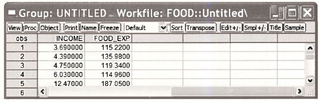
1.2. Checking summary statistics
In the definition file food.def we find variable definitions and summary statistics.
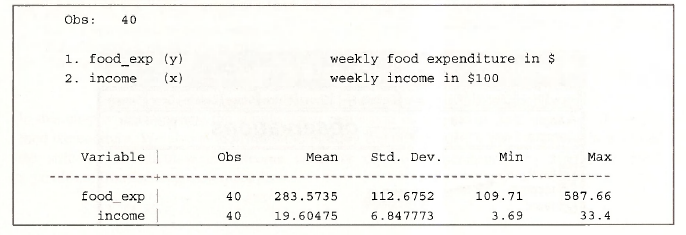
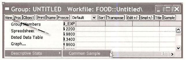
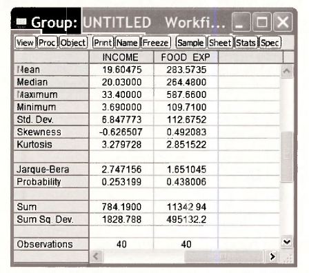
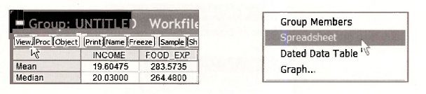
To verify that the workfile we are using agrees, select View/Descriptive Stats/Common Sample.
The resulting summary statistics agree with the information in the food.de/which assures us that we have the correct data.
To return to the spreadsheet view, select View/Spreadsheet
1.3. Saving a group
It is often useful to save a particular group of variables that are in a spreadsheet. From within the Group screen select Name and then assign an Object Name. Click OK.
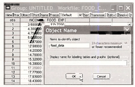
The new object in the workfile is a Group named FOOD DATA.

2. PLOTTING THE FOOD EXPENDITURE DATA
With any software there are several ways to accomplish the same task. We will make use of EViews “drop-down menus” until the basic commands become familiar. Click on Quick/Graph

In the dialog box type the names of the variables with the x-axis variable coming first!
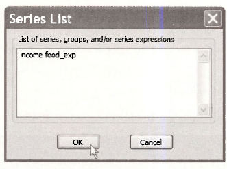
In the Graph Options box select Scatter from among the Basic graphs.

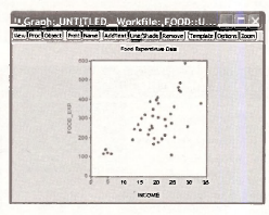
A plot appears, to which we can add labels and a title.

2.1. Enhancing the graph
While the basic graph is fine, for a written paper or report you it can be improved by
- adding a title
- changing vertical axis scale
These tasks are easily accomplished. To add a title, click on AddText on the Graph menu.

In the resulting dialog box you will be able to add a title, specify the location of the title, and use some stylistic features.
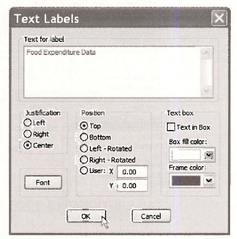
To have the title centered at the top click the appropriate options and type in the title. Click OK.
To alter the vertical axis so that it begins at zero, click on Options on the Graph Menu

Click on the Axes/Scale tab, select the Left Axis and Scale option in the drop down box. Choose User specified in the Left axis scale method. Enter 0 and 600 as the Min and Max values. Click OK.
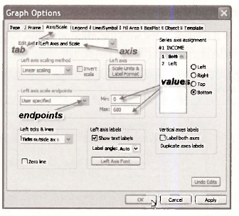
To change the “empty circles” used in the graph to “filled circles”, again choose Options, but select the Line/Symbol tab.
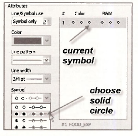
Click on Symbol pattern and choose the style you want. Note that other options are available. Click OK. The resulting graph is now
Explore the other tabs on the Options menu to see all the features.
2.2. Saving the graph in the workfile
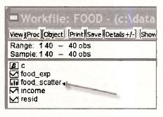
To save the graph, so that it remains in the workfile, click on Name, then enter a name. Note that separate words are not allowed, but separating words with an underscore is an alternative.

In the workfile, you will find an icon representing the graph just created
2.3. Copying the graph to a document
As is usual with Windows based applications, we can copy by clicking somewhere inside the graph, to select it, then Ctrl+C. Or in the main window click on Edit/Copy

The dialog box that shows up allows you to choose the file format. Switch to your word processor and simply paste the graph (Ctrl+V) into the document.
To save the graph to disk, select the Object button on the Graph menu.

Select View Options/Save graph to disk. In the resulting dialog box you have several file types to choose from, and you can select a name for the graph image.
2.4. Saving a workfile
You may wish to save your workfile at this point. If you select the Save button on the workfile menu the workfile will be saved under its current name food.w/1. It might be better to save this file under a new name, so that the original workfile remains untouched. Select File/Save As on the EViews menu and select a simple but informative name.

We will name it food_chap02.wfl
3. ESTIMATING A SIMPLE REGRESSION
To estimate the parameters b\ and b-> of the food expenditure equation, we select Quick/Estimate Equation from the EViews menu.
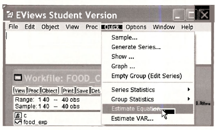
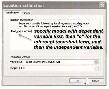
In the Equation Specification dialog box, type the dependent variable FOOD EXP (the y variable) First, C (which is EViews notation for the intercept term, or constant), and then the independent variable INCOME (the x variable). Note in the Estimation settings window, the Method is Least Squares and the Sample is 1 40. Click OK.
The estimated regression output appears. EViews produces an equation object in its default Stats view. We can name the equation object to save it permanently in our workfile by clicking on Name in the equation’s toolbar. We have named this equation FOOD_EQ.
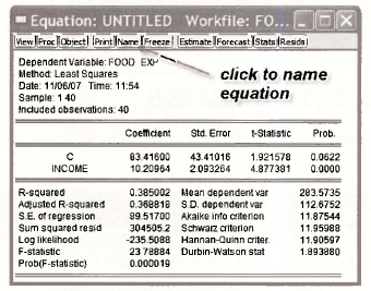
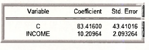
Note the estimated coefficient bi, the intercept in our food expenditure model is recorded as the coefficient on the variable C in EViews. C is the EViews term for the constant in a regression model. Note that we cannot name any of our variables C since this term is reserved exclusively for the constant or “intercept” in a regression model. Our EViews output shows b\ — 83.4160. The estimated value of the slope coefficient on the variable weekly income (X) is b2 – 10.2096, as reported in POE, Chapter 2.3.2. The interpretation of b2 is: for every $100 increase in weekly income we estimate that there is about a $10.21 increase in weekly food expenditure, holding all other factors constant.
In the workfile window, double click on the vector object C. It always contains the estimated coefficients from the most recent regression.
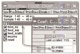
The vector RESID always contains the least squares residuals from the most recent regression. We will return to this shortly.
3.1. Viewing equation representations
One EViews button that we will use often is the View button in a regression window
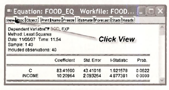
On the drop down menu list click Representations
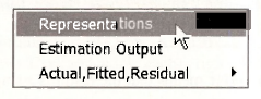
The resulting display shows three things:
- The Estimation Command is what can be typed into the command line to obtain the equation results.
- The Estimation Equation that shows the coefficients and how they are linked to the variables on the equation’s right side: C( 1) is the intercept and C(2) is the slope
- The Substituted Coefficients displays the fitted regression line.

To return to the regression window click Stats.
3.2. Computing the income elasticity
As shown in equation (2.9) of POE the income elasticity is defined to be

which is then implemented by replacing unknowns by estimated quantities,
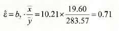
We can use EViews as a “calculator” by simply typing into the command line

then pressing Enter. The word scalar means that the result is a single number. An icon appears in the workfile,

Double-click in the shaded area, and in the lower left comer of the EViews screen you will find the result

While this gives the answer, there is something to be said for using the power of EViews to simplify the calculations. EViews saves the estimates from the most recent regression in the workfde. They are obtained by double clicking the “β” icon
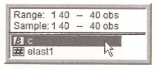
These coefficients can be accessed from the array @coefs. Also, EViews has functions to compute many quantities. The arithmetic mean is computed using the function @mean. Thus the elasticity can also be obtained by entering into the command line
scalar elast2 = @coefs(2)*@mean(income)/@mean(food_exp)
The result is slightly different than the first computation because in the first we used “rounded off’ values of the sample means.
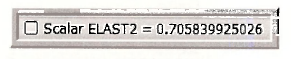
Because the array @coefs is not permanent, you may want to save the slope estimate as a separate quantity by entering the commands
scalar b2 = @coefs(2)
scalar elast3 = b2*@mean(income)/@mean(food_exp)
However, the coefficient array can always be retrieved if the food equation has been saved and named. Recall that we did save it with the name FOOD_EQ. By saving the equation we also save the coefficients, which can by retrieved from the array FOOD_EQ.@coefs.
scalar elas = food_eq.@coefs(2)*@mean(income)/@mean(food_exp)
We have some surplus icons in our workfile now. Keep B2 and ELAS. To clean out the other elasticties, highlight (hold down Ctrl and click each), right-click in the blue area, and select Delete. Save the workfile.
4. PLOTTING A SIMPLE REGRESSION
Select Quick/Graph from the EViews menu. In the Series List dialog box enter INCOMEand FOOD EXP.

On the Type tab select Scatter
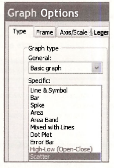
In the Details section, using the Fit lines drop down menu, select Regression Line.
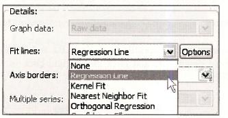
Edit the scale of the vertical axis, choose solid circles for data points, and add a title as shown in Section 2.2.1. Click inside the graph, enter Ctrl+C, OK, and then paste into a document using Ctrl+V. The graph should look like this.

Return to EViews and in the Graph window select the Name button and assign a name to this object, such as FITTED LINE.
5. PLOTTING THE LEAST SQUARES RESIDUALS
The least squares residuals are defined as

As you will discover these residuals are important for many purposes. To view the residuals open the saved regression results in FOOD_EQ by double clicking the icon.
5.1. Using View options
Within the equation FOOD_EQ window, click on View then Actual, Fitted, Residual. There you can select to view a table or several graphs.
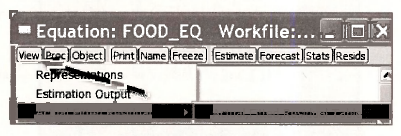
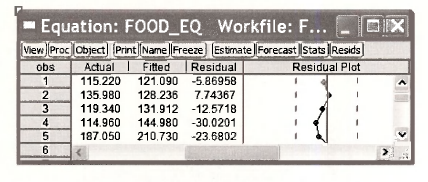
If you select Actual, Fitted, Residual Table you will see the values of the dependent variable y, the predicted (fitted) value of y, given by y = b, + b2x and the least squares residuals, along with a plot.
5.2. Using Resids plot
Within the object FOOD_EQ you can navigate by selecting buttons. Select Resids.
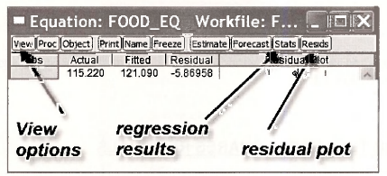
The result is a plot showing the least squares residuals (lower graph) along with the actual data (FOOD EXP) and the fitted values. When using this plot note that the horizontal axis is the observation number and not INCOME. In this workfile the data happen to be sorted by income, but note that the fitted values are not a straight line. When examining residual plots, a lack of pattern is consistent with the assumptions of the simple regression model.

5.3. Using Quick/Graph
To create a graph of the residuals against income we can use the fact the EViews saves the residuals from the most recent regression in the series labeled RESID. Click on Quick/Graph. In the dialog box enter INCOME (x-axis comes first) and RESID.
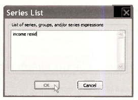
Choose the Scatter plot. The resulting plot shows how the residuals relate to the values of income.

Save this plot by selecting Name and assigning RESIDUAL_PLOT.
5.4. Saving the residuals
To save these residuals for later use, we must Generate a new variable (series). In the workfile screen click Genr on the menu.
[Genr|
In the resulting dialog box create a new variable called EHAT that contains the residuals
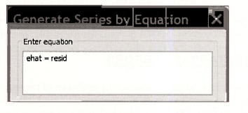
Click OK. Alternatively, simply type into the command line
series ehat = resid
6. ESTIMATING THE VARIANCE OF THE ERROR TERM
The estimator for σ2, the variance of the error term is

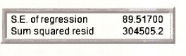
where Sum squared resid is the EViews name for the sum of squared residuals. The square root of the estimated error variance is called the Standard Error of the Regression by EViews,

Open the regression equation we have saved as FOOD_EQ. Below the estimation results you will find the Standard Error of the Regression and the sum of squared least squares residuals.
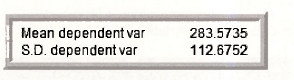
Also reported are the sample mean of the y values (Mean dependent variable)

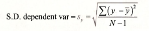
The sample standard deviation of the y values (S.D. dependent var) is
These are
7. COEFFICIENT STANDARD ERRORS
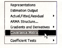
The estimated error variance is used to construct the estimates of the variances and covariances of the least squares estimators as shown in POE equations (2.20)-(2.22). These estimated variances can be viewed from the FOOD_EQ regression by clicking on View/Covariance Matrix
The elements are arrayed as
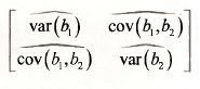
In EViews they appear as
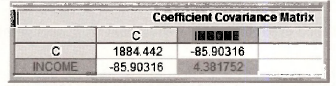
The highlighted value is the estimated variance of b2. If we take the square roots of the estimated variances, we obtain the standard errors of the estimates. In the regression output these standard errors are denoted Std. Error and are found right next to the estimated coefficients.
8. PREDICTION USING EVIEWS
There are several ways to create forecasts in EViews, and we will illustrate two of them.
8.1. Using direct calculation
Open the food equation FOOD_EQ. Click on View/Representations. Select the text of the equation listed under Substituted Coefficients. We can choose Edit/Copy from the EViews menubar, or we can simply use the keyboard shortcut Ctrl+C to copy the equation representation to the clipboard. Finally, we can paste the equation into the command line.
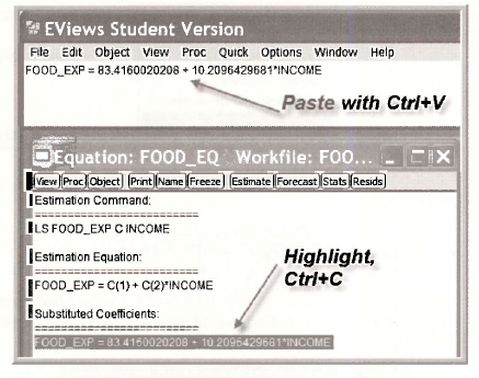
To obtain the predicted food expenditure for a household with weekly income of $2000, edit the command line to read
scalar FOOD_EXP_HAT = 83.4160020208 + 10.2096429681*20
Press Enter. The resulting scalar value is

which is correct to more decimals than the value 287.61 we report in Chapter 2.3.3b.
8.2. Forecasting
A more general, and flexible, procedure uses the power of EViews. In order to predict we must enter additional x observations at which we want predictions. In the main workfile window, double-click Range. This workfile has an Unstructured/Undated structure. Change the number of observations to 43.
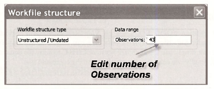
Click OK. EViews will check with you to confirm your action.

Next, double-click on INCOME in the main workfile to open the series, and click the Edit+/- button in the series window, which puts EViews in edit mode.
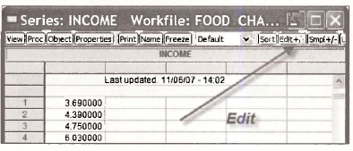
Scroll to the bottom and you see NA in the cells for observations 41-43. Click the cell for observation 41 and enter 20. Enter 25 and 30 in cells 42 and 43, respectively. When you are done, click the Edit+/- button again to turn off the edit mode.
Now we have 3 extra INCOME observations that do not have FOOD EXP observations. When we do a regression EViews will toss out the missing observations, but it will use the extra INCOME values when creating a forecast.
To forecast, first re-estimate the model with the original data. This step is not actually necessary, but we want to illustrate a point. Click on Quick/Estimate Equation. Enter the equation. Note in the dialog box that the Sample is 1 to 43.

The estimation results are the same, and EViews tells us that the Included observations are 40 after adjustments. The 3 observations with not values for FOOD EXP were discarded.
To forecast with the estimated model, click on the Forecast button in the equation window.
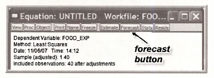
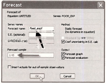
The Forecast dialog box appears. EViews automatically assigns the name FOOD_EXPF to the forecast series, so if you want a different name enter it. The Forecast sample is 1 to 43. Predictions will be constructed for the 40 samples values and for the 3 new values of INCOME. For now, ignore the other options. Click OK.
A graph appears showing the fitted line for observations 41-43 along with lines labeled ±2 S.E. We will discuss these later. To see the fitted values themselves, in the workfile window, double click on the series named FOOD EXPF and scroll to the bottom.
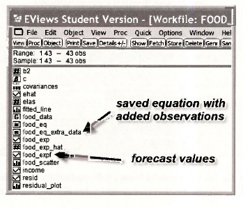
There you see the three forecast values corresponding to incomes 20, 25 and 30. The value in cell 41 is 287.6089, which is the same predicted value we obtained earlier in Chapter 2.3.3b.
While this approach is somewhat more laborious, by using it we can generate forecasts for many observations at once. More importantly, using EViews to forecast will make other options available to us that simple calculations will not.
Source: Griffiths William E., Hill R. Carter, Lim Mark Andrew (2008), Using EViews for Principles of Econometrics, John Wiley & Sons; 3rd Edition.
The post The Simple Linear Regression Model by using EViews appeared first on HKT Consultant.
]]>The post Interval Estimation and Hypothesis Testing by using EViews appeared first on HKT Consultant.
]]>For the regression model y = β1 +β2x + e, and under assumptions SR1-SR6, the important result that we use in this chapter is given in equation (3.3) of POE.
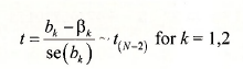 ’
Using this result we can show that the interval bk ± tcse(bk) has probability 1-a of containing the true but unknown parameter p*, where the “critical value” tc from a /-distribution such that P(t>tc) = P(t<-tc) = a/2
To construct interval estimates we will use EViews’ stored regression results. We will also make use of EViews built in statistical functions. For each distribution (see Function reference in EViews Help) four statistical functions are provided. The two we will make use of are the cumulative distribution (CDF) and the quantile (Inverse CDF) functions.
The for the /-distribution the CDF is given by the function @ctdist(x,v). This function returns the probability that a /-random variable with v degrees of freedom falls to the left of x. That is,

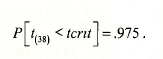
The quantile function @qtdist(p,v) computes the critical value of a /-random variable with v degrees of freedom such that probability p falls to the left of it. For example, if we specify tc=@qtdist(.975,38), then
To construct the interval estimates we require the least squares estimates bk and their standard errors se(bk). After each regression model is estimated the coefficients and standard errors are saved in the arrays @coefs and @stderrs. However they are saved only until the next regression is run, at which time they are replaced. If you have named the regression results, as we have (FOOD_EQ) then the coefficients are saved as well, with the names food_eq.@coefs and food_eq.@stderrs, respectively.
1.1. Constructing the interval estimate
Since we have estimated only one regression we can use the simple form for the saved results. Thus @coefs(2) = b2 and @stderrs(2) = se(b2). To generate the 95% confidence interval [b2 – tcse{b2), b2 + tcse(b2)\ enter the following commands in the EViews command window, pressing the <Enter> key after each:
scalar tc = @qtdist(.975,38)
scalar b2 = @coefs(2)
scalar seb2 = @stderrs(2)
scalar b2_lb = b2 – tc*seb2
scalar b2_ub = b2 + tc*seb2
These scalar values show up in the workfile with the symbol #. For example, the value of the lower bound of the interval estimate is

1.2. Using a coefficient vector
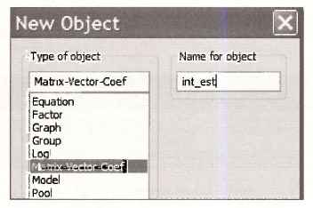
While the above approach works perfectly fine, it may be nicer for report writing to store the interval estimates in an array and construct a table. On the main EViews Menu select Objects/New Object
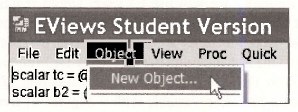
We will create a Matrix-Vector-Coef named INT EST
It will be a coefficient vector that has 2 rows and 1 column
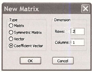
Click OK, and the empty array appears. Instead of all that pointing and clicking, you can simply enter on the command line
coef(2) int_est
Now, enter the commands
int_est(1) = @coefs(2) – @qtdist(.975,38)*@stderrs(2)
int_est(2) = @coefs(2) + @qtdist(.975,38)*@stderrs(2)
Here we have used the EViews saved results directly rather than create scalars for each elements. The vector we created is
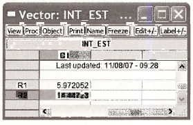
Click on Freeze and then Name. We chose the name B2 INTERVAL ESTIMATE and it looks like this:
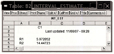
The advantage of this approach is that the contents can be highlighted, copied (Ctrl+C) and pasted (Ctrl+V) into a document. The resulting table can be edited as you like

2. RIGHT-TAIL TESTS
2.1. Test of significance
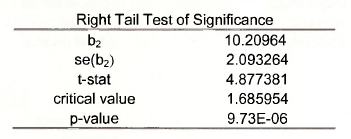
To test the null hypothesis that (32 = 0 against the alternative that it is positive (> 0), as described in Chapter 3.4.1a of POE, requires us to find the critical value, construct the /-statistic, and determine the /7-value.
- If we choose the a = .05 level of significance, then the critical value is the 95th percentile of the /(3g) distribution.
- The /- statistic is the ratio of the estimate bi over its standard error, se(b2).
- The /7-value is the area to the right of the calculated /-statistic (since it is a right-tail test). This value is one minus the cumulative probability to the left of the /-statistic.
The simplest set of commands is (do not type the comments in italic font)
scalar tc95 = @qtdist(.95,38) t-critical right tail
scalar tstat = b2/seb2 t-statistic
scalar pval = 1 – @ctdist(tstat,38) right-tail p-value
Alternatively, use the vector approach outlined in the previous section
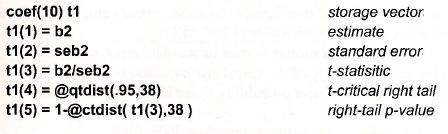
Use the results of this vector to construct a table, such as
2.2. Test of an economic hypothesis
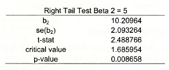
To test the null hypothesis that β2 < 5 against tl alternative β2 > 5 the same steps are executed, except for the construction of the t-statistic.
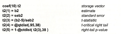
Yielding
3. LEFT-TAIL TESTS
3.1. Test of significance
To test the null hypothesis that β2 > 0 against the alternative that it is negative (< 0) requires us to find the critical value, construct the t-statistic, and determine the p-value.
- If we choose the a = .05 level of significance, then the critical value is the 5th percentile of the t(38) distribution.
- The t- statistic is the ratio of the estimate b2 over its standard error, se(b2).
- The p-value is the area to the left of the calculated /-statistic (since it is a left-tail test). This value is given by the cumulative probability to the left of the t-statistic.
The simplest set of commands is (do not type the comments in italic font)

Alternatively
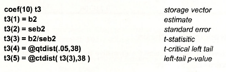
Yielding
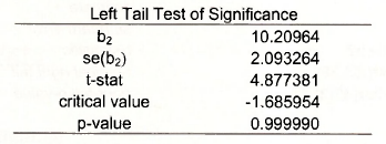
Note that we fail to reject the null hypothesis in this case, as expected.
3.2. Test of an economic hypothesis
To test the null hypothesis that β2 >12 against the alternative that β2 < 12, we use the same steps as above, except for the construction of the t-statistic.
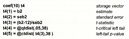
Yielding,
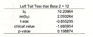
The t-statistic value -.85 does not fall in the rejection region, and the p-value is about .20, thus we fail to reject this null hypothesis.
4. TWO-TAIL TESTS
4.1. Test of significance
The two tail test of the null hypothesis that β2 = 0 against the alternative that β2 # 0 we require the same test elements
- If we choose the a = .05 level of significance, then the right-tail critical value is the 97.5- percentile of the f(38) distribution and the left tail critical value is the 2.5-percentile.
- The t- statistic is the ratio of the estimate bi over its standard error, se(£>->).
- The p-value is the area to the left of minus the absolute value of the calculated t-statistic plus the area to the right of the absolute value of the calculated test statistic (since it is a two-tail test). This value is given by the cumulative probability to the left of the – |t-statistic| and l – the cumulative probability to the right of |t-statistic|.
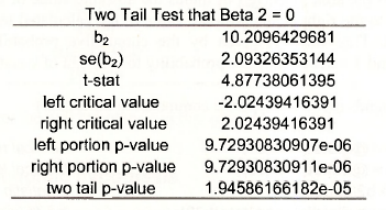
The two tail p-value is

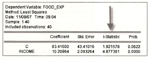
The test is carried out by EViews each time a regression model is estimated. If we examine FOOD_EQ, in the column labeled t-statistic is the ratio of the Coefficient to Std. Error. The column labeled Prob. contains the two-tail p-value for the test of significance. Note that the very small p-value is rounded to zero (to 4 places). For practical purposes this is enough since levels of significance below .001 are hardly ever used.
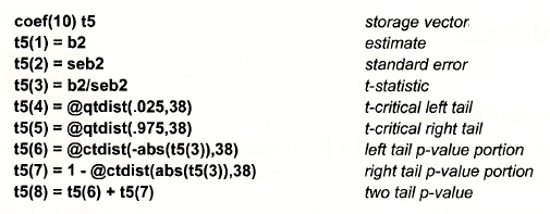
To use the coefficient vector approach
The result is as follows. Here we have copied the results from EViews at the highest precision to show that the p-value works out to be the same as reported above.
4.2. Test of an economic hypothesis
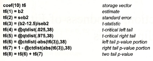
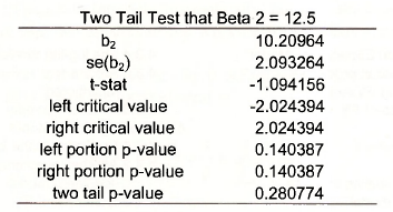
To test the null hypothesis that β2 = 12.5 against the alternative β2 # 12.5 the steps are the same as those above, except for the construction of the t-statistic.
Which yields
Source: Griffiths William E., Hill R. Carter, Lim Mark Andrew (2008), Using EViews for Principles of Econometrics, John Wiley & Sons; 3rd Edition.
The post Interval Estimation and Hypothesis Testing by using EViews appeared first on HKT Consultant.
]]>