Evaluating and Testing the Research Model

Evaluating and testing a model does not simply mean testing the hypotheses or relationships between the model’s concepts or variables one after the other, but also judging its internal global coherence.

1. Qualitative Methods

In some studies, researchers want to test the existence of a causal relationship between two variables without having recourse to sophisticated quantitative methods (such as those presented in the second part of this section). In fact, situations exist in which the qualitative data (resulting from interviews or docu­ments) cannot be transformed into quantitative data or is insufficient for the use of statistical tools. In this case, researchers identify within their data the arguments that either invalidate or corroborate their initial hypothesis about the existence of a relationship between two variables. They then establish a decision-making rule for determining when they should reject or confirm their initial hypothesis. To establish such a rule, one needs to refer back to the exact nature of the researcher’s hypotheses (or propositions). Zaltman et al. (1973) identify three types of hypothe­ses that can be tested empirically: those that are purely confirmable, those that are purely refutable and those that are both refutable and confirmable.

• Hypotheses are considered to be purely confirmable when contrary argu­ments, discovered empirically, do not allow the researcher to refute them. For example, the hypothesis that ‘there are opinion leaders in companies that change’, is purely confirmable. In fact, if researchers discover contrary argu­ments, such as companies changing without opinion leaders, this does not mean they should refute the possibility of finding such leaders in certain cases.
• Hypotheses are considered to be purely refutable when they cannot be confirmed. A single negative instance suffices to refute them. Asymmetry therefore exists between verifiability and falsifiability). For example, the hypo­thesis ‘all companies which change call upon opinion leaders’ is purely refutable. In fact, finding just one case of a company changing without an opinion leader is sufficient to cast doubt on the initial hypothesis. Universal propositions form part of this group of hypotheses. Indeed, there are an infi­nite number of possibilities for testing such propositions empirically. It is, therefore, difficult to demonstrate that all possible situations have been thought of and empirically tested.

The testing of such hypotheses is not undertaken directly. One needs to derive sub-hypotheses from the initial hypothesis and then confirm or refute them. These sub-hypotheses specify the conditions under which the initial proposition will be tested. For example, from the hypothesis ‘all com­panies which change call upon opinion leaders’ one derives the hypothesis that ‘type A companies call upon opinion leaders’ and the auxiliary hypo­thesis that ‘type A companies have changed’. It is therefore possible, to iden­tify clearly all the companies belonging to group A and test the derived hypothesis among them. If one company in the group has not called on an opinion leader in order to implement change then the derived hypothesis is refuted and, as a result, so is the initial hypothesis. If all type A companies have called upon opinion leaders when instituting change, the derived hypothesis is then confirmed. But the researcher’s cannot conclude that the initial hypothesis is also confirmed.

• The final group consists of hypotheses that are both confirmable and refutable. As an example, let us consider the hypothesis ‘small companies change more often than large ones’. To test such a hypothesis, it suffices to calculate the frequency with which small and large companies change, then compare these frequencies. The presence of a single contrary argument does not systematically invalidate the initial hypothesis. Conversely, as Miles and Huberman (1984a) point out, one cannot use the absence of contrary evidence as a tactic of decisive confirmation.

To move from testing a relationship to testing a model, it is not enough to juxtapose the relationships between the model’s variables. In fact, as we saw in the introduction to this section, we must ascertain the model’s global coher­ence. Within the framework of a qualitative method, and particularly when it is inductive, researchers face three sources of bias that can weaken their con­clusions (Miles and Huberman, 1984a):

• The holistic illusion: according events more convergence and coherence than they really have by eliminating the anecdotal facts that make up our social life.
• Elitist bias: overestimating the importance of data from sources who are clear, well informed and generally have a high status while underestimating the value of data from sources that are difficult to handle, more confused, or of lower status.
• Over-assimilation: losing one’s own vision or ability to pull back, and being influenced by the perceptions and explanations of local sources (Miles and Huberman, 1984a).

The authors propose a group of tactics for evaluating conclusions, ranging from simple monitoring to testing the model. These tactics permit the researcher to limit the effects of earlier bias.

2. Quantitative Methods

Causal models illustrate a quantitative method of evaluating and testing a causal model. However, evaluating a model is more than simply evaluating it statistically. It also involves examining its reliability and validity. These two notions are developed in detail in Chapter 10. We have, therefore, chosen to emphasize a system that is the most rigorous method for examining causal rela­tionships, and permits the researcher to increase the global validity of causal models. This is experimentation.

2.1. Experimental methods

The experimental system remains the favored method of proving that any vari­able is the cause of another variable. Under normal conditions, researchers test­ing a causal relationship have no control over the bias that comes from having multiple causes explaining a single phenomenon or the bias that occurs in data collection. Experimentation gives researchers a data collection tool that reduces the incidence of such bias to the maximum.

Experimentation describes the system in which researchers manipulate vari­ables and observe the effects of this manipulation on other variables (Campbell and Stanley, 1966). The notions of factor, experimental variables, independent variables and cause are synonymous, as are the notions of effect, result and dependent variables. Treatments refer to different levels or modalities (or combinations of modalities) of factors or experimental variables. An experi­mental unit describes the individuals or objects that are the subject of the experimentation (agricultural plots, individuals, groups, organizations, etc.). In experimentation, it is important that each treatment is tested on more than one experimental unit. This basic principle is that of repetition.

The crucial aim of experimentation is to neutralize those sources of variation one does not wish to measure (that is, the causal relationship tested). When researchers measure any causal relationship, they risk allocating the observed result to the cause being tested when the result is, in fact, explained by other causes (that is, the ‘confounding effect’). Two tactics are available for neutraliz­ing this confounding effect (Spector, 1981). The first involves keeping constant those variables that are not being manipulated in the experiment. External effects are then directly monitored. The limitations of this approach are imme­diately obvious. It is impossible to monitor all the non-manipulated variables. As a rule, researchers will be content to monitor only the variables they con­sider important. The factors being monitored are known as secondary factors and the free factors are principal factors. The second tactic is random allocation, or randomization. This involves randomly dividing the experimental units among different treatments, in such a way that there are equivalent groups for each process. Paradoxically, on average, the groups of experimental units become equivalent not because the researcher sought to make them equal according to certain criteria (that is, variables), but because they were divided up randomly. The monitoring of external effects is, therefore, indirect. Randomization enables researchers to compare the effects of different treatments in such a way that they can discard most alternative explanations (Cook and Campbell, 1979). For example, if agricultural plots are divided up between different types of soil treatment (an old and a new type of fertilizer), then the differences in yields cannot result from differences in the amount of sunshine they receive or the soil composition because, on the basis of these two criteria, the experimental units (agricultural plots) treated with the old type of fertilizer are, on average, comparable with those treated with the new type. Randomiza­tion can be done by drawing lots, using tables of random numbers or by any other similar method.

All experimentation involves experimental units, processing, an effect and a basis for comparison (or control group) from which variations can be inferred and attributed to the process (Cook and Campbell, 1979). These different ele­ments are grouped together in the experimental design, which permits researchers to:

• select and determine the method for allocating experimental units to the dif­ferent processes
• select the external variables to be monitored
• choose the processes and comparisons made as well as the timing of their observations (that is, the measurement grades).

There are two criteria researchers can use to classify their experimental pro­gram, with a possible crossover between them. They are the number of princi­pal factors and the number of secondary (or directly monitored) factors being studied in the experimentation. According to the first criterion, the researcher studies two or more principal factors and possibly their interactions. A factor analysis can either be complete (that is, all the processes are tested) or it can be fractional (that is, certain factors or treatments are monitored). According to the second criterion, total randomization occurs when there is no secondary factor (that is, no factor is monitored with a control). The experimental units are allo­cated randomly to different treatments in relation to the principal factors studied (for example, if there is one single principal factor which comprises three modalities, it constitutes three treatments, whereas if there are three principal factors with two, three and four modalities, that makes 2x3x4, or 24 treatments). When there is a secondary factor, we refer to a random bloc plan. The random bloc plan can even be complete (that is, all the treatments are tested within each bloc) or it can be incomplete. The experimental system is the same for total ran­domization, except that experimental units are divided into subgroups accord­ing to the modalities of the variable being monitored, before being allocated randomly to different treatments within each subgroup. When there are two sec­ondary factors, we refer to Latin squares. When there are three secondary fac­tors, they are Greco-Latin squares, and when there are four or more secondary factors they are hyper-Greco-Latin squares. The different systems of squares require that the number of treatments and the number of modalities, or levels of each of the secondary factors, are identical.

In the experimental systems presented earlier, experimental units were ran­domly allocated to treatments. Agricultural plots are easier to randomize than individuals, social groups or organizations. It is also easier to conduct randomi­zation in a laboratory than in the field. In the field, researchers are often guests whereas, in the laboratory, they can feel more at home and often have virtually complete control over their research system. As a result, randomization is more common in the case of objects than people, groups or organizations and is more often used in the laboratory than during fieldwork.

Management researchers, who essentially study people, groups or organi­zations and are the most often involved in fieldwork, rarely involve themselves in experimentation. In fact, in most cases, they only have partial control over their research system. In other words, they can choose the ‘when’ and the ‘to whom’ in their calculations but cannot control the spacing of the stimuli, that is, neither the ‘when’ or the ‘to whom’ in the treatments, nor their randomiza­tion, which is what makes true experimentation possible (Campbell and Stanley, 1966). This is ‘quasi-experimentation’.

Quasi-experimentation describes experimentation that involves treatments, measurable effects and experimental units, but does not use randomi­zation. Unlike experimentation, a comparison is drawn between groups of non­equivalent experimental units that differ in several ways, other than in the presence or absence of a given treatment whose effect is being tested. The main difficulty for researchers wishing to analyze the results of quasi-experimentation is trying to separate the effects resulting from the treatments from those due to the initial dissimilarity between of groups of experimental units.

Cook and Campbell (1979) identified two important arguments in favor of using the experimental process in field research. The first is the growing reti­cence among researchers to content themselves with experimental studies in a controlled context (that is, the laboratory), which often have limited theoretical and practical relevance. The second is researcher dissatisfaction with non­experimental methods when making causal inferences. Quasi-experimentation responds to these two frustrations. Or, more positively, it constitutes a middle way, a kind of convergence point for these two aspirations. From this point of view, there is bound to be large-scale development in the use of quasi­experimentation in management.

So far in this section we have been talking essentially about drawing causal inferences using variables manipulated within the framework of an almost com­pletely controlled system. In the following paragraphs, we focus on another family of methods that enable causal inferences to be made using data that is not necessarily experimental. These are causal models.

2.2. Statistical methods

There are three phases in the evaluation and testing of causal models: identifi­cation, estimation and measurement of the model’s appropriateness.

Every causal model is a system of equations in which the unknowns are the parameters to be estimated and the values are the elements of the variance/covariance matrix. Identifying the causal model involves verifying whether the system of equations which it is made of has zero, one or several solutions. In the first instance (no solution), the model is said to be under­identified and cannot be estimated. In the second case (a single solution), the model is said to be just identified and possesses zero degree of freedom. In the third case (several solutions), the model is said to be over-identified. It possesses several degrees of freedom, equal to the difference between the number of ele­ments in the matrix of the variances/covariance (or correlations) and the num­ber of parameters to be calculated. If there are p variables in the model, the matrix of the variances/covariance is counted as p(p + 1)/2 elements and the matrix of correlations p(p – 1)/2 elements. These two numbers have to be compared with those of the parameters to be calculated. However, in the case of complex models, it can be difficult to determine the exact number of parameters to be calculated. Fortunately, the computer software currently available automatically identifies the models to be tested and displays error messages when the model is under-identified.

Statistically testing a causal model only has interest and meaning when there is over-identification. Starting from the idea that the S matrix of the observed variances/covariance, which is calculated on a scale, reflects the true X matrix of the variances/covariance at the level of all of the population, one can see that, if the model’s system of equations is perfectly identified (that is, the number of degrees of freedom is null), then the C matrix reconstituted by the model will equal the S matrix. However, if the system is over-identified (that is, the number of degrees of freedom is strictly positive) then the correspondence will probably be imperfect because of the presence of errors related to the sample. In the latter case, estimation methods permit researchers to calculate parameters which will approximately reproduce the S matrix of the variances/covariance observed.

After the identification phase, the model’s parameters are estimated, most often using the criterion of least squares. A distinction can be drawn between simple methods (unweighted least squares) and iterative methods (maximum likelihood or generalized least squares, etc.). With each of these methods, the researcher has to find estimated values for the model’s parameters that permit them to minimize an F function. This function measures the difference between the observed values of the matrix of the variances/covariance and those of the matrix of variances/covariance predicted by the model. The parameters are assessed iteratively by a non-linear optimization algorithm. The F function can be written as follows:

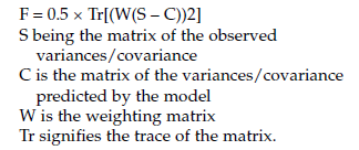
In the method of unweighted least squares, W equals I, the matrix identity. In the method of generalized least squares, W equals S – 1, the inverse of the matrix of the observed variances/covariance. In the method of maximum like­lihood, W equals C – 1, the inverse recalculated at each iteration of the matrix of variances/covariance predicted.

After the estimation phase, the researcher has to verify the model’s appro­priateness in relation to the empirical data. The appropriateness of a model in relation to the empirical data used to test it is greater when the gap between the matrixes of predicted and observed variances and covariance (S) is weak. However, the more parameters the model has to be estimated, the greater the chance that the gap will be reduced. For this reason, evaluation of the model must focus as much on the predictive quality of the variance/covariance matrix as on the statistical significance of each of the model’s elements.

Causal models offer a large number of criteria to evaluate the degree to which a theoretical model is appropriate in relation to empirical data. At a very general level, we can distinguish between two ways of measuring this appropriateness:

• the appropriateness of the model can be measured as a whole (the Khi2 test, for example)
• the significance of the model’s different parameters can be measured (for example, the t test or z test).

Software proposing iterative estimation methods, such as generalized least squares or maximum likelihood, usually provide a Khi2 test. This test compares the null hypothesis with the alternative. The model is considered to be accept­able if the null hypothesis is not rejected (in general, p > 0.05). This runs con­trary to the classic situation in which models are considered as acceptable when the null hypothesis is rejected. As a result, Type II errors (that is, the probability of not rejecting the null hypothesis while knowing it is false) are critical in the evaluation of causal models. Unfortunately, the probability of Type II errors is unknown.

In order to offset this disadvantage, one can adopt a comparative rather than an absolute approach, and sequentially test a number of models whose differ­ences are established by the addition or elimination of constraints (that is, ‘nested models’). In fact, if researchers have two models, one of which has added constraints, they can test the restricted model versus the more general model by assessing them separately. If the restricted model is correct, then the difference between the Khi2 of the two models approximately follows a Khi2 distribution and the number of degrees of freedom is the difference in degrees of freedom between the two models.

It is, however, worth noting two major limitations of the Khi2 test:

• When the sample is very big, even very slight differences between the model and the data can lead to a rejection of the null hypothesis.

• This test is very sensitive to possible discrepancies from a normal distribution.

As a result, other indices have been proposed to supplement the Khi2 test. The main software packages, such as LISREL, EQS, AMOS or SAS, each offer more than a dozen. Certain of these indices integrate explained variance percentage allowances. Usually, the models considered to be good models are those whose indices are above 0.90. However, the distribution of these indices is unknown and one should therefore exclude any idea of testing appropriate­ness statistically. A second category groups together a set of indices which take real values and which are very useful for comparing models that have different numbers of parameters. It is usual, with these indices, to retain as the best those models whose indices have the lowest values.

In addition to these multiple indices for globally evaluating models, numer­ous criteria exist to measure the significance of models’ different parameters. The most widely used criterion is that of ‘t’ (that is, the relation between the parameter’s value and its standard deviation). This determines whether the parameter is significantly non-null. Likewise, the presence of acknowledged statistical anomalies such as negative variances and/or determination coeffi­cients that are negative or higher than the unit are naturally clear proof of a model’s deficiency.

All in all, to meet strict requirements, a good model must present a satisfac­tory global explanatory value, contain only significant parameters and present no statistical anomalies.

In general, the use of causal models has come to be identified with the com­puter program LISREL, launched by Joreskog and Sorbom (1982). As renowned as this software might be, we shouldn’t forget that there are other methods of estimating causality which may be better suited to certain cases. For example, the PLS method, launched by Wold (1982), does not require most of the restric­tive hypotheses associated with use of maximum likelihood technique generally employed by LISREL (that is, a large number of observations and multi­normality in the distribution of variables). Variants of the LISREL program, such as CALIS (SAS Institute, 1989) or AMOS (Arbuckle, 1997), and other programs such as EQS (Bentler, 1989) are now available in the SAS or SPSS software pack­ages. In fact, the world of software for estimating causal models is evolving constantly, with new arrivals, disappearance and, above all, numerous changes.

Source: Thietart Raymond-Alain et al. (2001), Doing Management Research: A Comprehensive Guide, SAGE Publications Ltd; 1 edition.