Piece-rates and time-rates in the firm

1. Payment Schedules, Moral Hazard and Effort

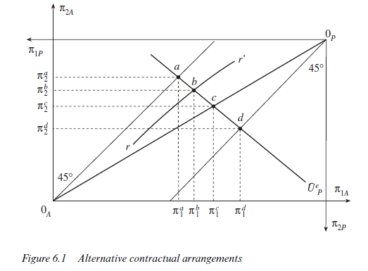
Although employment contracts were discussed at various points in Chapter 5, it will be useful to reinterpret some of the principal-agent results in terms of more conventional concepts. Our analysis thus far has been conducted with the aid of a simple box diagram, with each point in the box representing a ‘contract’. Implicitly, therefore, each point represents a primitive ‘payment schedule’ or ‘incentive structure’. It determines what contractually accrues to the agent or employee in given circumstances. Suppose, as we did initially in section 4 of Chapter 5, that only the final outcome of the employees’ effort is observable, then each point in the box diagram can be interpreted as implying a payment schedule made up of a time-rate and a piece-rate. Consider Figure 6.1 in which we reproduce a box diagram with the risk-neutral employer’s indifference curve U_p^e. Along U_p^e we identify four possible contractual positions labelled a, b, c and d respec­tively. The locus rr’ which will just induce effort e from the risk-averse employee is drawn through point b. Point c lies on a diagonal drawn through the principal’s origin and the agent’s origin. Point a and point d are on the agent’s certainty line and the principal’s certainty line respectively.

Each of the identified contracts can be illustrated in a different way in Figure 6.2. Along the horizontal axis in Figure 6.2 is measured the actual outcome and along the vertical axis the payment to the employee. Since there are only two possible outcomes in our simple formulation, each con­tract point in Figure 6.1 is represented by two points in Figure 6.2. Thus, contract a in Figure 6.1 is equivalent to the two points a’ and a” in Figure 6.2. A straight line drawn through these two points is horizontal, indicat­ing that the payment to the employee is independent of the outcome. This can therefore be regarded as a pure time-rate system. The employee receives a certain payment n^a₁ = π^a₂. Interpreting the ‘outcomes’ measured by the dimensions of the box as referring to particular intervals of time (in Chapter 5 it might have been a year, since there we were discussing the size of the harvest, but here we could regard the outcomes as applying to weekly intervals), n^a₁ =π^a₂ would represent a weekly wage.

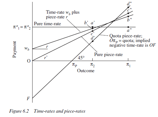
As was seen in Chapter 5, a weekly wage in the context of total lack of observability of effort would not produce the required work incentives. To induce effort, the employee had to take some risk, and in the present context this implies an element of piece-rate payment. Point b in Figure 6.1 transfers to the two points b’, b” in Figure 6.2. A straight line through these points cuts the vertical axis at w_b. It is therefore possible to interpret the contract at b in Figure 6.1 as a combination of a time-rate or weekly wage w_b and a payment per unit of outcome or piece-rate given by the slope of the line through b’ and b”. Designate the slope of this line as r, then the payment to the employee = w_b + rπ where π is the actual outcome. This

payment schedule will just induce the risk-averse employee to exert effort e, as was seen in Chapter 5. A contract at point c in Figure 6.1, it will be recalled, would involve risk-sharing losses relative to point b and (given the assumption of only two effort levels, zero and e) would result in no com­pensating increase in effort. The contract at c lies on the diagonal through the origins of the box and thus implies that the agent is paid the same pro­portion of the outcome, whichever outcome occurs. There is thus no time­rate at all but just a pure piece-rate, as shown in Figure 6.2 by the straight line through the origin. Of course there is no reason in principle why a con­tract at c, and hence a pure piece-rate, might not be an efficient solution to the contractual problem, given the right circumstances (the degree of risk aversion of the employee, the cost of effort to the employee, the effect of effort on the probability of π, and so forth).

Indeed, although a risk-averse employee will never, according to the results of Chapter 5, be observed accepting a contract at d (since another contract will exist preferred by both employer and employee), a risk-neutral employee may do so. The resulting payment schedule is shown as the straight line through d’ and d in Figure 6.2. Note that the implied time­rate is now negative and represents the ‘franchise fee’ discussed in the last chapter. It should not be concluded, however, that this fee has actually to be paid to the employer in the form of cash for the incentive structure to be operating. The fee can be paid ‘implicitly’ by effectively forgoing any reward over a certain range of outcomes, and hence paying the fee ‘in kind’ to the employer. Thus a piece-rate system can involve a ‘quota’ below which the employee receives nothing. In the case of the contract at d, the employee receives whatever is produced,⁷ but only above the quota ^rn_p.

The fact that only two outcomes were assumed to be possible meant that the various incentive structures could be represented by points lying along the straight lines in Figure 6.2. In the general case, where any number of outcomes might occur and effort levels can vary continuously, there is absolutely no reason to suppose that the efficient contract will imply a linear incentive structure. Indeed, the informational and computational requirements involved in ‘calculating’ the best contract will be formidable and the result could be a highly complex structure. Once more, therefore, we are led back to the basic arguments of Chapters j and 2 and the propo­sition that bounded rationality and other information problems will imply continual experiment rather than perfectly stable ‘solutions’. Stiglitz (1975) recognises this point and argues in terms reminiscent of Alchian (1950) or even Hayek (1937, 1945) that: ‘If there are large and significant advantages of one contractual arrangement over another, firms that ‘discover’ (this) will find they can increase profits and the particular contractual arrange­ment will be imitated. Thus, it might be argued that there is an evolution­ary tendency of the economy to gravitate to the contractual arrangements analysed here’ (p. 556). Stiglitz proceeds to investigate the properties of linear payment schedules where employees are risk averse and employers are risk neutral, and derives results which may be intuitively understood in the context of the model presented in Chapter 5: ‘The piece rate is higher the smaller the risk, the lower the risk aversion, and the higher the supply elasticity of effort (the greater the incentive effects)’ (p. 560).

In other words, if output is very closely related to effort and only weakly influenced by chance elements (the risk is small) the payment schedule will emphasise the piece-rate, and the time-rate will be low. By opting for piece­rates, the employee does not expose him- or herself to great risk but there is a clear advantage in providing incentives to effort. The impact of risk aversion also accords with a priori expectations. Where, as in Stiglitz’s model, the outcome alone is observable, contracts which induce effort will involve the employee in some risk (unless of course there is no environ­mental risk and π = π(e)). As we saw in Chapter 5, the risk-sharing losses were worth incurring provided that the incentive effects were big enough. There we were considering a case in which effort could take only two values, but where effort can vary continuously the efficient contract will be so adjusted that the additional risk-sharing losses associated with inducing an extra unit of effort from the employee are just equal to the marginal benefits derivable from the extra effort. Clearly, the more risk averse the employee the greater will be the risk-sharing losses involved in any given modifications of the incentive structure away from time-rates towards piece-rates. Marginal risk-sharing losses will exceed marginal benefits from greater effort sooner as the importance of piece-rates is increased, and higher risk aversion is therefore expected to favour the time-rate. By a similar process of reasoning it is clear that for any given degree of risk aver­sion the marginal benefits of a move towards piece-rates will be higher the greater the resulting incentive effects, and thus large incentive effects favour the piece-rate. A final conclusion from Stiglitz’s analysis also accords with the results of our simple framework: ‘If individuals are perfectly well informed about their own abilities’ (that is, they know the cost of effort and the effect on the probability distribution of outcomes) ‘and there are no other sources of risk’ (or people are risk neutral) ‘then equilibrium will entail . . . auctioning off the jobs to the highest bidder; that is, a non­positive time rate’ (p. 563). This corresponds, of course, to our conclusion that with risk-neutral employees the incentive structure d’d” in Figure 6.2 will be efficient.

2. Payment Schedules, Adverse Selection and Worker Sorting

Choice of incentive structure will also have an impact on the quality of worker recruited when this quality or ‘ability’ is unobservable and adverse selection is a problem. A simple demonstration that firms with higher piece­rates tend to prevail when the ability level of workers is unobservable can be derived by assuming that workers’ (observable) output is closely corre­lated to their ‘ability’. If, subject to meeting a competitive profit constraint, firms can offer different contracts (such as those in Figure 6.2) high piece­rate firms will dominate low piece-rate firms. Suppose we have just two qualities of worker. Effort is either zero, in which case nothing is produced, or one. For effort level one, quality-1 workers will produce output π₁ and quality 2 workers will produce π₂. Higher output is thus linked to higher quality not to higher effort. The worker knows his or her productivity with certainty. Clearly quality-1 workers will receive a higher payment under a quota piece-rate than under the other schedules (compare d” with c” and b” in Figure 6.2) while for quality-2 workers it will be the other way around (compare b’, c’ and d’).⁸ Low-quality workers will therefore offer their ser­vices to firms with low-powered incentives and high-quality workers will seek employment in firms with high-powered incentives.

Assume now that the distance OF (the payment to the principal) in Figure 6.2 represents a competitive payment for capital per worker which all firms must achieve. Firms offering schedules c’c” or b’b” would make a loss. They would attract quality-2 workers and their output would be π₂. The output available for paying the worker after the demands of capital had been satisfied would be π₂ – k_P which equals vertical distance d’π₂, but the amount promised to the worker would be greater than this, implying a loss per worker of vertical distance c’d’ or b’d’. To make profits, firms offering payment schedules c’c” or b’b” require quality-1 workers, but quality-1 workers prefer to work in firms offering payment schedule d’d”.

Clearly, the argument sketched in the previous paragraphs abstracts from many important considerations. However, it produces some clear predic­tions. A firm moving from time-rates to piece-rates under conditions in which individual output is measurable at fairly low cost would expect to encounter two effects. Work effort is expected to rise as shown in section 2.1 and the average quality of the workforce is also expected to rise as high- quality workers choose to work in firms offering piece-rates. Lazear (2000b) reports strong support for both of these predictions from a study of Safelite; a US autoglass installer which switched from hourly wages to piece-rates in the mid-1990s. An overall rise in productivity of 44 per cent could be divided into two components – a rise in the productivity of exist­ing workers as their effort responded to the new incentives and a rise due to the recruitment of workers attracted by the new regime.

Source: Ricketts Martin (2002), The Economics of Business Enterprise: An Introduction to Economic Organisation and the Theory of the Firm, Edward Elgar Pub; 3rd edition.