Accepting (or Rejecting) Hypotheses: Objective Criteria

At this stage, the experiment has yet to be conducted and the experimenter has yet to decide which of the two hypotheses he should favor. But the “favoring” is not a matter of fancy; it can­not be decided arbitrarily. The consequences of accepting one or the other of the possible hypotheses should be logically analyzed through the medium of statistical quantities. An outline of such an analysis follows.

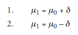
Firstly, μ1 = μ0 means that the property in question, as obtained by changing one or more parameters, remains unal­tered. This is the null hypothesis, and the two forms of the alter­nate hypothesis are

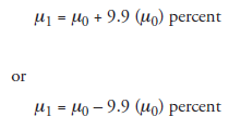
For one thing, in either form, we cannot say that the improve­ment will be acknowledged only if it is exactly δ. A little less or a little more should be acceptable. But how much is “a little”? Sup­-pose the intended improvement in the design is 10 percent. Then, should

whichever is applicable, be rejected as no improvement, thus, treated like the null hypothesis? Doing so amounts to committing a β error. How can this error be avoided despite the numbers tempting us to make it? Bound as the experimenter is to work in the domain of probability, not certainty, we may say that he should increase the probability, as much as possible under the circumstances, of not making the error. It is in this form that probability enters the scene. Furthermore (this is important), in the above relations we have used μ1, the population mean of the improved property, as if it would be accessible. If we could directly measure it, we could compare it with the value μ0 + δ or μ0 – δ, as the case may be, see how close μ1 is to the designed values, and make the appropriate decision. But what would become accessible, after performing the experiment, is only the sample mean, X1, which, at best, is only an approximation to μ1. Now the question is reduced to, How will X1, obtained after the improvement, be related to μ0, which is available before the experiment? Further, X1 being the mean for a definite number of elements in the sample, what should be the size of the sample?This becomes anot her question in designing the experiment. The
logic and statistics involved in answering such questions are quite complex and beyond the scope of this book. In this context, the
experimenter, assumed to be not a trained statistician, would do well to take on faith, without insisting on proofs, the procedural steps, including do’s and don’ts, formulated by statisticians. Four typical designs, each with a distinct set of experimental situations frequently encountered, are discussed as follows.

Source: Srinagesh K (2005), The Principles of Experimental Research, Butterworth-Heinemann; 1st edition.