With minor variations, the following are the steps for designing simple comparative experiments:
- Identify whether O is known for the responses represented in μ0. If it is not known, more calculations will be required, as we will see later in the procedure.
- State the null and the alternate hypotheses to represent the experimental conditions. Identify whether the alternate hypothesis is “one sided” or “two sided.”
- Make a decision on the appropriate risk factors, α and β.
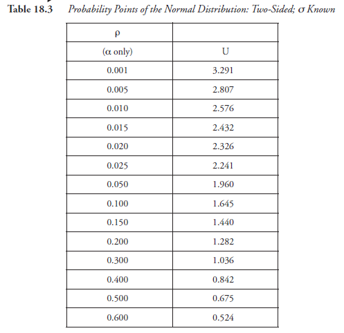
- Go to Table 18.2 if “one sided” or to Table 18.3 if “two sided”; these tables list the “probability points” appropriate to the situations in the experiment.
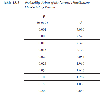
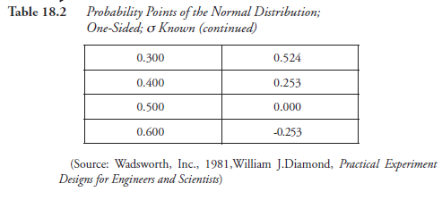
Corresponding to the numerical values selected for α and β above, find the probability points, symbolized here as Uα and Uβ.
- Compute N, the size of the sample, to be tested for evaluating μ1.
- Compute X, the criterion numbers.
For computing both N and X, formulas are prescribed appropriate to the set of experimental conditions.
Steps that come after this point depend on the “responses” from the experiment attempting to effect the intended improvement, represented by fip, but the procedure for using these responses, which are yet to come, can and should be planned in advance.
- Experiment to obtain a sample of N
- Calculate the mean, X1, of the improved responses, represented by μ1, using the prescribed formula, appropriate to the experimental conditions.
- Compare the numerical values of X1 with that of X.
- Decide to accept or reject one or the other of the hypotheses, as prescribed, again, depending on the experimental conditions.
The above procedure for planning the experiment is used as the “template” in which each of the steps, 1 to 10, represents a particular function. For example, step 5 is assigned to calculating N, the sample size. When a particular step, for instance 5, in turn requires two or more substeps, 5a, 5b, etc. are assigned to such substeps. And, if a particular step, for instance 4, requires two or more iterations, they are shown with subscripts, (4)j, (4)2, etc. Unless otherwise mentioned, the numbers confirm to this scheme in the following discussion including examples.
1. Criterion Values
For solving problems in designing experiments, statisticians have provided the formulas needed to compute the numerical values of what are known as criterion values. The factors involved in the formulas are
σ the standard deviation of one or both populations, as required
N the sample size
δ the minimum acceptable improvement as used in the alternate hypothesis
Uα , Uβ the probability points (also known as the standard deviates) to be found in the appropriate statistical tables
Formulas for computing the criterion values for different sets of experimental situations vary. For a specific set of situations, after computing, the criterion value is kept ready to be compared with the sample mean of the improved responses (the dependent variable), to be obtained after the experimental runs are performed.
Situation Set 1
- It is a test for simple comparison, before and after the improvement.
- The alternate hypothesis is Ha: μ1 > μ0.
- μ0 for population before improvement is known.
- σ, the standard deviation of the measurements used for μ0, is known.
With this set of situations, which is more often encountered than others, an example follows:
Example 1:
The following experiment is designed to allay the concerns of an engineer who is required to supervise the performance of a heating plant in a public building. The independent variable available to him is the operating temperature, which can be set as required by a thermostat. The dependent variable is the pressure in a steam vessel, an important component of the heating plant. With the operating temperature set at 300°F, the average pressure reading is 250 psi; the standard deviation is known to be ten. The engineer is facing the demand from his crew to increase the pressure to 260 psi. Based on his experience with the plant and its operation, the engineer predicts that setting the temperature at 350°F will accomplish this goal.
Procedure:
- σ, the standard deviation, is known to be ten.
Note: Dimensional units associated with the numbers are suppressed to conform to the format (and brevity) of the hypotheses.
- State the hypotheses:
Null hypothesis, H0: μ1 = μ0
Change in the pressure planned: 10
Alternate hypothesis, Ha: μ1 = μ0 + 10
This is a one-sided hypothesis.
- Decide the risk factors.
The risks involved are considered normal. Values, very often used in such analysis, are chosen.
α = 0.05, β = 0.10
- Go to Table 18.2.
Corresponding to a = 0.05, we find Ua = 1.645.
Corresponding to (3 = 0.10, we find Up = 1.282.
- Compute N, the sample size, using the formula prescribed for this set of conditions:
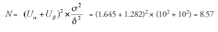
Take it as N = 9
- Compute X, the criterion number:
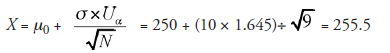
X is kept ready to be compared with Xj (yet to be evaluated after running the experiment), using nine samples.
The remaining part of the procedure is “road testing” the hypothesis.
- Conduct the experiment, which consists of setting the temperature to 350°F, followed (after sufficient time to stabilize the system) by recording several pressure readings over a reasonable length of time.
- Compute X1, the mean of nine randomly selected pressure readings from the population of such readings.
- Compare X1 with X
- Make decisions as recommended:
If X1 > X, accept the alternate hypothesis,
![]()
This means, put the plan into action; namely, set the operating temperature at 350°F, which “very likely” will result in the pressure of 260 psi, at the level it is required. “Very likely” here means a probability of 1 — 0.05, that is, 95 percent.
If, instead, X1 < X, accept the null hypothesis,
H0: μ1 = μ0, meaning that changing the operating temperature, likely, will not make any change in the pressure. “Likely” here means a probability of 1 – 0.1, that is, 90 percent.
Example 2:
Suppose the null hypothesis, as above, is the verdict of the design. What next? Does it mean that all is lost? Not at all. We can make another design and road test it again. Suppose we reflect that the quantum of increment in a pressure of nine units is quite adequate for the required purpose, then the new δ is nine instead of ten. The values of α and β can also be varied, meaning that the experimenter will accept the risk of making the α error and the βerror a t different probability levels. Let us say, for instance, that the new values of α and β chosen by the experimenter are both 0.05. Then, following the same steps of calculation, but with different numerical values, we have
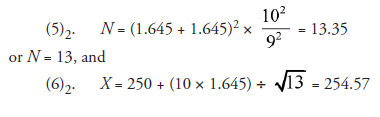
This means:
(7)2. After setting the temperature to 350°F, record the pressure readings over an extended period of time.
(8)2. Find X1, the mean of thirteen randomly selected pressure readings.
(9)2. Compare the new X1 with the new X, 254.57.
(10)2. Make the decision anew, with the same directions as before.
2. When σ Is Not Known
The process of design suffers a significant setback when a, the standard deviation of the population, is not known. Having to deal with one more unknown—in fact a vital one, σ—the degree of reliability is considerably lowered. But when such situations are encountered, a method worked out by statisticians is available to bypass the setback. Broadly, this method consists of the following additional steps:
- Finding N, the sample size, by two or more iterations.
- Finding the degree of freedom.
- Using t-distribution probability points in the second and later iterations.
- Calculating a sample (substitute) standard deviation to be used in place of the unknown standard deviation.
Situation Set 2
All the other situations are exactly the same as in Example 1 with the only difference that O is not known. The procedural steps are worked out, including the extra steps made necessary because of this difference.
Example 3:
- σ is not known.
- State the hypotheses:
H0: μ1 = μ0
H1: μ1 = μ0 + 10
- Choose the risk factors. α = 0.05 and β = 0.10
- Go to Table 18.2; look for Ua and Up
For α = 0.05, Uα = 1.645
For β = 0.10, Uβ = 1.282
- Compute N, the sample size.
N = (Uα + Uβ) × σ2 / δ2
The only term now unknown in the RHS (right hand side) of the equation is O, and that is what makes the difference in the steps and equations that follow.
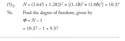
Suppose σ is specified in terms of δ (it is frequently done so), for instance, σ = (1.1) × δ. If it is not so specified, the experimenter
has the additional responsibility of deciding on a similar specification at his own discretion. Then,
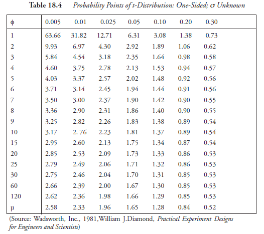
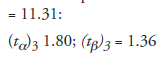
Note: The use of probability points for α and β, taken from Table 18.2, was good only for the first iteration, done above, for calculating N. For the second iteration, the probability points, in place of α and β, should be taken from Tables 18.4 and 18.5, which present t-distribution points, the values designated as tα and tβ. Table 18.4 provides values of tα and tβ when the alternate hyposthesis stated in step 2 is “one (single) sided.” Table 18.5 provides those values when the alternate hypothesis is “two double) sided.” Also, note that the t-distribution points are given in Tables 18.4 and 18.5, corresponding to Φ, the degree of freedom, a new parameter. These are the major differences.
Probability Points of t-Distribution; Two Sided; σ Unknown
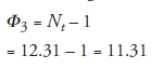
(4)2. Look up t-distribution points in Table 18.4, corresponding to Φ = 9.37 (interpolating):
![]()
(5)3. Compute the sample size again, this time using t-distribution points in place of Uα and Uβ; it is given by
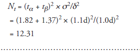
Note: The above value, 12.31, for sample size is the result of the third iteration. A fourth iteration is known to be a closer approximation, which can be obtained by repeating steps 5 to 4 to 5 again, using the corresponding t-points.
For instance,
(5b)2. Find the degree of freedom, given by
(4)3. Look for t-points in Table 18.4, corresponding to Φ :
(5)4. Compute sample size again:
![]()
The difference in sample size as computed by the fourth iteration is not significantly different from that by the third iteration; thus, usually the third iteration is considered quite adequate in most cases.
Now that the preceding procedural steps have been carried out with N = 12, the experiment is ready to test drive.
- Set the temperature at 350°F; after a reasonable length of time, record several pressure readings, x^ over an extended period.
- Find the mean of twelve randomly selected pressure readings, X1.
- Find the standard deviation of these readings, given by
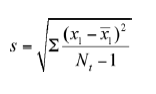
Note: s, calculated as above, will now be substituted in place of the standard deviation, s, which is not known. Now, we
are back on track, as if σ were known.
- Using S, the estimated standard deviation, compute the criterion value, given by
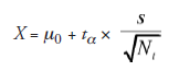
Note: Compare this equation with the parallel equation for case A (σ known). Notice ta in place of Ua, and Nt in place of N.
9. Compare X1 with X.
10. Make the decision:
If Xj > X, accept the alternate hypothesis,
H1: μ1 = μ0 + 10, meaning there is a 95 percent possibility that the pressure will increase to 260 psi.
If, instead, X1 < X, accept the null hypothesis, H0: μ1 = μ0, meaning there is a 90 percent possibility that the pressure will remain unchanged.
Source: Srinagesh K (2005), The Principles of Experimental Research, Butterworth-Heinemann; 1st edition.
4 Aug 2021
4 Aug 2021
4 Aug 2021
5 Aug 2021
5 Aug 2021
5 Aug 2021