Asking the questions and forecasting the likely answers from the experiment are done in the formal language of statistics. The question-answer formats are known as null and alternate hypotheses. These are described below.
1. Null Hypothesis in an Experiment
The term null connotes negation, that is, rejecting (or saying no to) a specific assertion. In the context of experimental research, the null hypothesis is used when the experimental data (which is represented by a sample) does not necessarily warrant a generalization (which represents the entire population) that an intended improvement in the dependent variable did not occur. The null hypothesis, H), is stated as
H0 : μ1 = μ0,
which is the symbolic way of saying that the independent variable, targeted to be improved, remains unchanged. The failure to improve may be the result of an unaccountable experimental (including sampling) error due to random influences. The experimenter then resorts to a decision-making criterion; for instance, if the probability of the effect of random influences is found to be less than 5 percent, he will reject the hypothesis that the data does not warrant generalization, meaning that the data then is worthy of generalization. The situation may be understood as follows: The experimenter starts with the “pessimistic approach” of saying that the specific data (in the form of a bunch of numbers of common significance) is not fully trustworthy and, hence, deserves to be scrapped. This is accepting the null hypothesis. Then, after careful deliberation in terms of statistical criteria, he may find, for instance, that there are fewer than one in twenty (5 percent) chances that random influences are responsible for what appears to be a meaningful variation that can be deciphered from the data. And so, in moderation, he will develop confidence in the data and make a decision that the data, after all, is not untrustworthy. This is rejecting the null hypothesis.
To the experimenter, the data is all-important. That is what he planned for and strove to get. Once the data is in hand, however, he does not accept it without subjecting it to the “acid test” of statistics, which consists of first taking the side of the critics, and then, only after examining the evidence, being convinced that there is overwhelming reason to move away from the critics and to take, instead, the side of the supporters. This is the most common and convenient path available to the experimenter as a way of developing confidence in his data. The experimenter, thus, states his null hypothesis in such a way that the rejection of the null hypothesis is what he hopes for.
There is in this path a parallel to the treatment of a crime suspect in the court of law. The starting point for the court is to assume that the person accused of the crime is innocent. The prosecutor is required to prove by appropriate evidence that this assumption is wrong. If the evidence is overwhelming against the assumption, the court will change the opinion it started with, that is, reject its own assumption. If, on the other hand, the evidence provided by the prosecutor is not overwhelming, the court will accept its own assumption as valid.
What we have referred to so far as “overwhelming evidence” is not the evidence that may be considered, for instance, as “105 percent strong.” There is no such thing in the domain of probability and statistics; there is nothing even “100 percent strong,” for then, we would be talking in terms of absolute certainty, which is contrary to statistical truth. The highest possible “strength” in probability approaches, but never reaches, 100 percent. Likewise, there is nothing like 0 percent strength either; the lowest strength approaches, but never reaches, 0 percent. In light of this, within the domain of probability, the data that lead toward accepting the null hypothesis are not to be considered totally worthless. The possibility is open to consider whether there is an alternate method by which the data can be subjected to scrutiny afresh. Appropriately named, there is such a thing as an alternate hypothesis.
But first let us look at and contrast the consequences of either rejecting or accepting the null hypothesis. The parallel that we have drawn between the null hypothesis in logic and the way the court of law deals with the crime suspect can be extended further. Despite all the care exercised by the legal system, it is not impossible that there will be cases in which innocent persons are declared guilty and punished and cases in which guilty persons are declared innocent and set free. In terms of logic, when the null hypothesis is rejected, even though it is true, it is similar to punishing an innocent person; it is called in logic a type I error. When the null hypothesis is accepted, even though in reality the hypothesis is false, it is called a type II error, which is similar to a guilty person going scot-free. Are the legal system and inferential logic, then, built on faulty foundations? Not quite. The possibility that such errors can occur should be attributed to the fact that the legal system and inferential logic are both based on probability, not certainty; the numerical value of probability can never be 1.0, for then certainty would have asserted itself in the place of probability.
2. Alternate Hypothesis
The phrase alternate hypothesis is deliberately used, with this significance: that if the null hypothesis is proved false, the alternate hypothesis is accepted automatically to be true without the need for a separate and independent proof. The two hypotheses, null and alternate, should be so stated that they conform to this understanding. Thus, the most general way the alternate hypothesis can be stated is
Ha : μ1 ≠ μ0
With the null hypothesis formulated asμ1 = μ0, the value of Ui is definite, since the experimenter knows the value of μ0 In contrast, with the alternate hypothesis formulated using the sign of inequality (“≠”), the value of μ1 is indefinite, meaning it may
be either less than μ0 or more than μ0. Such hypotheses are aptly termed two-sided alternate hypotheses. Stating the hypotheses, instead, in the two variations
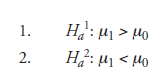
(in both cases the reference being μ0, and the focus of change being on μ1) will render them “one-sided,” though they will remain indefinite, meaning, in either case, the difference between μ1 and μ0 is not specified. And, in both the variations, μ1 can be an improvement over μ0. It may appear surprising that μ1 < μ0 is an alternate hypothesis, implying improvement, while the numerical value of the property is reducing. The explanation is simple: if the property under consideration is the life of ball bearings in hours, (1) is an improvement, hence the intention of the experimenter. If, instead, the property in question is the percentage of items rejected in the process of performing quality control for a manufactured product, then (2) is an improvement, hence, again, the goal of the experimenter.
As pointed out earlier, however, it is not enough to say there should be “some improvement” in the property. Planning the experiment requires that the degree of improvement should be specified. Then (1) and (2) above should be modified as
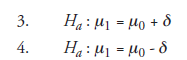
as the case may be.
3. Risks Involved: a and Errors
Occasioned by the facts that (j the null hypothesis will be accepted or rejected on the basis of the sample mean, not the population mean, and (2) the sample mean cannot be expected to be exactly equal to the population mean, it is reasonable not to expect absolute certainty in deriving the inference from the experimental results; there is always an element of risk involved. Relative to the null and alternate hypotheses, the risks are distinguished as follows:
- The experimenter accepts the alternate hypothesis (Ha) as true, that is, rejecting the null hypothesis, when, actually, the null hypothesis (H0) is true. In statistics, this is known as an alpha error, often simply indicated as
- The experimenter accepts the null hypothesis (H0) as true, when, actually, the alternate hypothesis (Ha) is true (and the null hypothesis is false). In statistics, this is known as a beta error, indicated as β.
We note that an experimenter cannot make both the errors together, for, as mentioned above, it is always either-or between the null and the alternate hypotheses. The risk of making either of the two errors is expressed in terms of probability. For instance, if it is assumed in the design that the experimenter is likely to make an α error of 0.1, then there is a 0.1 (100) = 10 percent chance of his accepting the alternate hypothesis as true, although, actually, the null hypothesis is true, and the chance of his making the correct decision of accepting the null hypothesis is reduced from 100 percent to (1 — 0.1) x 100 = 90 percent. Whether the probability so chosen should be 0.1, as mentioned above, or some other number (such as 0.16 or 0.09) is more or less a subjective decision, made by the experimenter, taking into consideration such factors as (1) the difference it makes, in terms of time and money involved, (2) the level of accuracy intended in the experiment, and (3) how critical the outcomes of the decision are, as applied to a real-life situation.
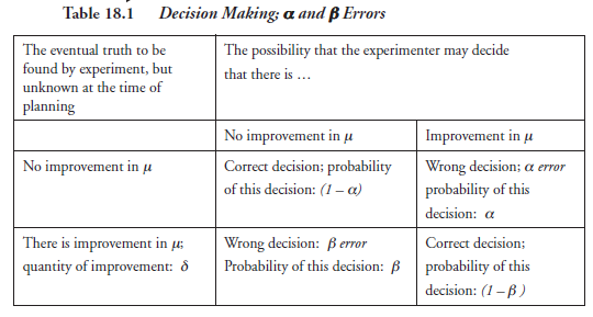
It is also possible that the experimenter will make the right decision in accepting either the null hypothesis or the alternate hypothesis, as the case may be. But here, again, that he may do so is not an absolute certainty; it is only a probability, however high it may be. Thus, we may think of there being four possibilities with the single-sided alternate hypothesis, each assigned the cor-responding probabilities. Table 18.1 shows these possibilities, with the following, normally accepted meanings for the symbols:
μ: the property that is meant to be improved by making certain changes in the related independent variables; understood to be the mean of a set of readings or measurements or calculated values, expressed as a number
δ: the number expressing the quantity or degree of improvement expected in μ
α: α error; a probability value (a number) assigned in the process of “designing” the experiment
β: β error; a probability value (a number) assigned in the process of designing the experiment
Referring to the example on ball bearings in Section 18.2.2, the value of 8, namely, one thousand hours of additional service life, should be specified as μ1 = μ0 + δ. Its significance lies in that, besides being a criterion to distinguish the null hypothesis from the alternate hypothesis, it relates to the sample size, discussed below, which, indeed, is another important factor to decide on in the process of planning. We note that formulating the null hypothesis is fairly easy: it is a statement to reflect that the effort to improve upon the given property is going to be fruitless. But the alternate hypothesis, as pointed out earlier, can be any one of the following statements:
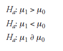
In these statements, μ0 and μ1 are the mean values of the property in question, meant to be obtained from the entire populations, μ0 from production before, and μ1 from the population after, the improvement. But in most (if not all) experiments, only the samples can be subjected to experimentation, not the entire populations. For instance, in the experimenton ball bearings, if it is in the plan to subject every one of the bearings made to the test in lab for its service life, there will be no bearings to sell. It is in this connection that the sample, and through that, the sample mean, X (to be distinguished from the population mean), of the property and the sample size enter into the design considerations.
4. Sample Mean X: Its Role in the Design
The sample mean, X (yet to be obtained and possible only after experimentation), and the population mean, μ0 (already known prior to experimenting), are logically related as follows:
- If X ≤ μ0, the property in question did not improve; hence, accept the null hypothesis.
- If X ≤ μ0 + δ, the property did improve per target; hence, accept the alternate hypothesis.
In either case, the decision is simple. But what if X is between μ0 and μ0 + δ? That is,
![]()
Depending on the closeness of X either to μ0 or to μ0 + δ, the situation could prompt the experimenter to accept either the null hypothesis or the alternate hypothesis.
5. Hypotheses Based on Other Parameters
We need to note that, depending on what the experiment sets out to “prove,” null and alternate hypotheses may often be stated in terms of other statistical parameters, such as standard deviation or variance, as below:
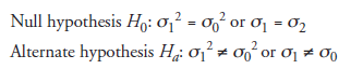
But in all the discussions that follow in this chapter, μ, the population mean, is used as the statistic of reference.
Source: Srinagesh K (2005), The Principles of Experimental Research, Butterworth-Heinemann; 1st edition.
Outstanding story there. What occurred after? Good luck!
Hi to every body, it’s my first go to see of this website; this web
site contains awesome and in fact good data designed for visitors.
Pretty! This has been a really wonderful article.
Thanks for supplying these details.
Wonderful post! We will be linking to this particularly great post on our website.
Keep up the good writing.
Very nice article, exactly what I was looking for.