As a way of preparing for factorial experiments with more than two factors, let us slightly modify the data in Table 8.5, using the “-1” and “+1” symbolism in place of “low” and “high” for the factor levels. The modification results in Table 8.6.
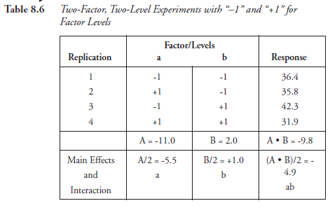
An explanation of the last two rows of this table is needed.
Evaluation of A was done as follows: Multiply each “response” value as found in the last column by either “-1” or “+1” as found in the a column in the corresponding row of the table. Then, add the resulting values together.
A = [36.4(—1)] + [35.8 (+1)] + [42.3 (-1)] + [31.9(+1)] = -11.0.
Similarly,
B = [36.4(-1)] + [35.8 (-1)] + [42.3(+1)] + [31.9(+1)] = +2.0.
The value of A • B is found on similar lines, with this difference; each response value is multiplied by the product of either “+1” or “-1” as found in column a and either “+1” or “-1” as found in column b. Sum of the four products thus obtained, shown below, is the value of A • B.
A • B= [36.4(-1) (-1)] + [35.8 (+1) (-1)] + [42.3(-1) (+1)] + [31.9(+) (+1)] = -9.8
The values of A, B, and A • B were derived using all four response values. The experiment yielding these responses could be formulated as y = f (a, b), wherein y gives the responses (the dependent variables), and a and b are two factors (independent variables) acting together. The effect of a on y, for instance, was tested for at two levels, a1 and a2, each requiring one replication. This means that two replications were necessary, yielding responses, to study the effect of a once. Four responses tested, thus, gives the effect of a, 4 ÷ 2 = 2 times. So, the main effect of a is obtained by dividing A by 2. The last row ofTable 8.6, thus, shows the main effect of a, that of b, and the interaction of a and b, respectively, symbolized as a, b, and ab.
The advantage of using the “-1” and “+1” symbolism for levels of factors must now be obvious to the reader. Evaluation of the main effects and the interaction can be done “mechanically,” without the need to penetrate the logic, and avoiding the possible confusion involved.
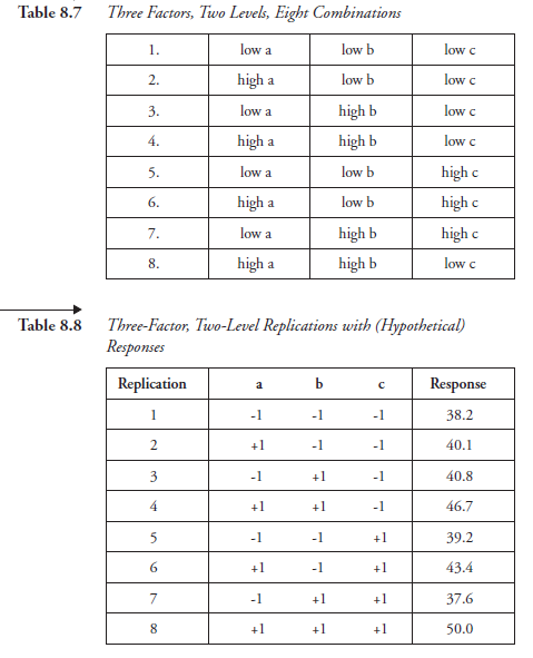
Now we may consider a full factorial of three factors, a, b, and c, each at two levels. The number of combinations is 23 = 8, shown in Table 8.7.
At this stage, the experimenter is expected to conduct the experiment with eight different factor combinations and to get a response for each combination. Table 8.8 shows the above combinations symbolized by “-1” and “+1,” respectively, for the “low” and “high” values of the three factors, with the corresponding hypothetical numerical values of the responses.
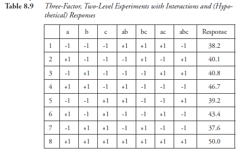
Among a, b, and c, we get the interactions ab, bc, ac, and abc. We may now extend the above table to include a column for each of these four interactions. As for the “—1” and “+1” signs required corresponding to each of these columns, a simple multiplication rule is all that is needed. For instance, in the third row of Table 8.8, we find a with “—1,” b with “+1,” and c with “—1” signs. On the same row, thus, ab will get a “—1” sign, as (—1) x (+1) = —1; bc will also get a “—1” sign, as (+1) x (—1) = —1; ac will get a “+1” sign, as (—1) x (—1) = +1; and abc will get a “+1” sign, as (—1) x (+1) x (—1) = +1. Working out such details can be done without the need for any further information. The data in Table 8.9 shows this method applied to all the eight rows.
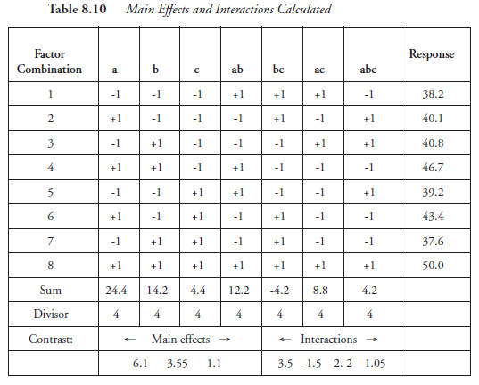
Using this table as the source, let us follow the method for calculating the main effects or interactions, together known as contrasts, each represented by a column within the matrix. We will do it for a to find the main effect of that factor. Following the procedure used with two factors in Table 8.6, now extending to three factors, we have
A = [(-1) (38.2) + (+1) (40.1) + (-1) (40.8) + (+1) (46.7) + (1) (39.2)+ (+1) (43.4) + (-1) (37.6) + (+1) (50.0)] = 24.4. The sum, 24.4, represents four responses at “low” levels and four responses at “high” levels of a. As two responses together, one at “low” and one at “high” levels of a, are required to know the effect of a once, the sum, 24.4, needs to be divided by four to get the “average effect” of a. The values of such sums for all seven columns, and the values of contrasts, obtained by dividing each by four (referred to as the divisor), are shown in Table 8.10.
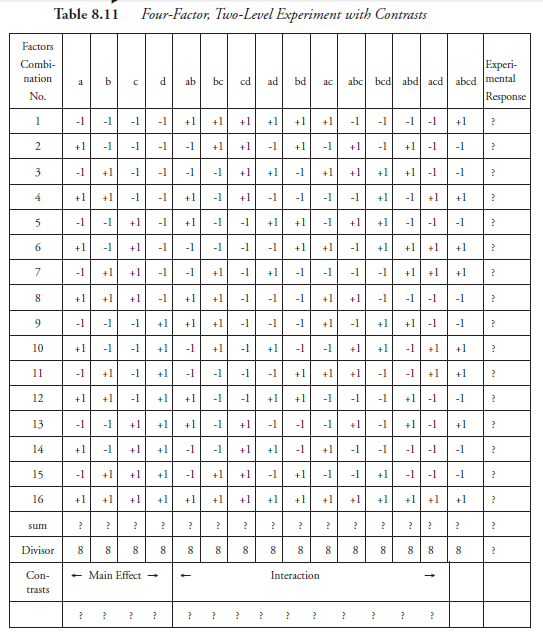
Thus far, we have shown how three factors may be represented. We will now go one step further and demonstrate how a matrix can be generated to represent four factors, a, b, c, and d, each at two levels. Then, the number of factor combinations is given by 24 = 16. Table 8.11 shows the combinations and interactions, together constituting the matrix, in terms of “-1” and “+1”
The “pattern” procedure required to generate the matrix for even larger numbers of factors must now be obvious to the reader. We point out a few noticeable features:
- The column corresponding to the first factor has “-1” and “+1” alternating one by one as we go down, factor combinations one to sixteen. (Note: There is no need to prioritize or establish an order among factors; they may be taken in any order.)
- Such alternating for the second factor/column is two by two; for the third factor/column it is four by four; for the fourth factor/column it is eight by eight.
Based on these observations, the pattern can be formulated as shown in Table 8.12.
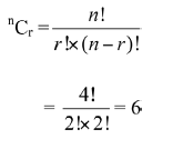
For the four columns in Table 8.11, each one representing one factor, the interactions are obtained by multiplying the corresponding “—1” and “+1” symbols, representing the factor levels, along the rows (across the columns). The number of interactions between any two factors, given by the number of combinations of two factors at a time among the four factors is
and these are ab, bc, cd, ad, bd, and ac. The interaction among these factors, given by the combination of three factors at a time among four factors is
![]()
These are abc, bcd, abd, and acd. The interaction among all four factors is, of course, given by one combination, abcd. Thus, there are 4 + 6 + 4 + 1 = 15 columns, each yielding a contrast, four contrasts of main effects, and eleven contrasts of interac-tions. With the four combinations shown in Table 8.6, there are three contrasts. With the eight combinations in Table 8.10, there are seven contrasts. With the sixteen combinations in Table 8.11, there are fifteen contrasts. We may, by induction, generalize that the number of contrasts will be equal to the number of combinations, minus one.
The reader should notice here that in each column, there are as many “—1” symbols as there are “+1” symbols. This feature follows in any matrix, however big it may be.
Now, if we have the numerical values of the responses obtained by experimentation, corresponding to each of the sixteen factor combinations, we can create a column next to the matrix, as shown in Table 8.11. The values of the main effect of the four factors and eleven interactions, together with fifteen contrasts, can each be evaluated simply by adding the sixteen products obtained by multiplying “—1” or “+1” in a given row of the column to the corresponding response value on the same row. In place of each response and each contrast, the values of these being unknown, a “?” mark is registered.
Source: Srinagesh K (2005), The Principles of Experimental Research, Butterworth-Heinemann; 1st edition.
5 Aug 2021
5 Aug 2021
5 Aug 2021
4 Aug 2021
4 Aug 2021
5 Aug 2021