Response of Multifactor Experiments

Whereas results of single-factor or one-factor-at-a time experi­ments can usually be compiled as y = fx), the response to multi­factor experiments needs a different treatment for analysis. We will start in this chapter with the simplest situation: two factors, at two levels each. We further assume that the factors are quanti­tative. But to keep the analysis adaptable to several different situ­ations, we will

1. Not identify the factors by their properties or dimensional units
2. Identify the factors only by names, as a, b, c, and so forth
3. Identify the levels of the factors by one of the many ways that we have mentioned earlier, namely, either as low and high ; — and + ; or a1 or a2 for a (and similarly for b, c, and so on), as this is convenient when there are only two levels

4. Record the responses as hypothetical quantities (for illustration) devoid of dimensional units

Table 8.5 shows the replication results of all combinations possible (full factorial) with two factors, a and b, with a at two levels, a1 and a2, and b at two levels, b1 and b2. The number of combinations is given by l^f = 2² = 4.

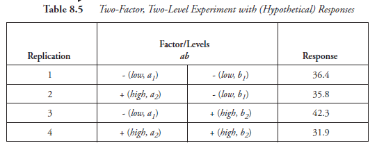
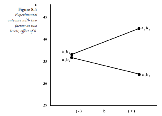
Figure 8.4 is the graphical presentation of the results shown in the second column of Table 8.5 for the change in a. The reader should also note that while the low level of a (ai) is shown first, then the high level (a₂), from left to right on the abscissa, there is no need to have a scale, and thus, one is not used. On the other hand, a scale is required for the ordinates, as these measure the responses in quantities as given in the last column of Table 8.5. Restricting our focus to Figure 8.4, we can measure the main effect of a as follows: factor a is changed from low (ai) level to high (af level, once with bi and another time with bj, each of these changes having caused a difference in the response. Consid­ering that there are two such changes, the effect of a (changing from aj to af) is given by the mean of the two differences: (response with a2 minus response with a1. That is,

Effect of a = [(35.8 – 36.4) + (31.9 – 42.3)] – 2 = -5.5

The negative sign, of course, should not be a surprise. As we mentioned earlier, the response could be a “loss” in a business; the negative sign then is an “improvement”! This same numerical value, intact with the sign, can be obtained if we now associate the “-” and the “+” signs in the a column of the table (the second column) with the corresponding numerical values of the response column (the fourth column). That is,

Effect of a = [-36.4 + 35.8 -43.3 + 31.9] – 2 = -5.5

Herein lies the advantage of using “-” and “+” signs instead of “low” and “high” or aj and a2, respectively. On the same lines as Figure 8.4, we can now represent the effect of b on the responses. The same four numbers in the last column of Table 8.5 now get assigned to “low” and “high” in the b (the third) column of the table. The result is shown in Figure 8.5. The effect of b can now be calculated, as shown above, by simply assigning the “-” and “+” signs of the b column in Table 8.5 to the corresponding numerical values for response in the last column. Thus,

Effect of b = [-36.4 – 35.8 + 42.3 + 31.9] – 2 = 1.0

Before we proceed further to deal with more involved situa­tions, we need to take note of two definitions, related to the graphical presentations in Figures 8.4 and 8.5.

1. The effects we have computed above for factors a and b are known as the main effect because each refers to the primary function of that factor as an independent variable, somewhat as if it were the only factor acting upon the dependent variable.

Usually, the symbols a and b are also used for the main effects of the corresponding factors as well.

2. In either figure, the line showing the effect of a and that showing the effect of b are nonparallel. In Figure 8.4, the lines actually cross each other. Such a situation is referred to as observation of an inter­action between the two factors a and b. In Figure 8.5, though the lines are nonparallel, there is no interaction within the experimental limits of the factors. If the two lines in Figure 8.4 were parallel, there would be no chance of their crossing each other, whatever the experimental limits of the vari­ables. This situation would be referred to as no interaction.

Now, what is the significance of interaction between the two factors a and b? It is an indication that a given factor fails to pro­duce the same effect on the response at different levels of the other factor. In Figure 8.4, for instance, at low levels of b (b^, the effect of a is

a = 35.8 – 36.4 = -0.6

and at high levels of b {b2}, the effect of a is

a = 31.9 – 42.3 = -10.4

This means that the effectiveness of a as an independent vari­able is sensitive to the amount of b that is coexisting and acting as another independent variable.

The extent of interaction, where it exists, is measurable. In our designation in Figure 8.4, it is referred to as the a • b interac­tion and is often symbolized as ab. The magnitude of the interac­tion, by definition, is half the difference between the two effects of a: the first at a high level of b (b2) and the second at a low level of b (bi). That is,

ab = [(31.9 – 42.3) – (35.8 – 36.4)] + 2 = -4.9

As a cross-check, suppose we now calculate the ba interaction, meaning the change in the effectiveness of b with the presence of a at different levels. At a high level of a (a2)

b = (31.9 – 35.8) = -3.9

and, at a low level of a (a₁)

b = 42.3 – 36.4 = 5.9

Then,

ba = [-3.9 – 5.9] + 2 = -4.9

As is to be expected, the extent of interaction is the same; that is, ab = ba.

We have shown earlier that multifactor experiments are more efficient than one-factor-at-a-time experiments. Here is yet another advantage of multifactor experiments: the aspect of interaction between factors could never be traced in a one-factor-at-a-time experiment.

Source: Srinagesh K (2005), The Principles of Experimental Research, Butterworth-Heinemann; 1st edition.