Fractional Factorials

Having arrived at the logical end point for discussing full-facto­rial experiments with four factors, we need to reflect on what lies ahead. We mentioned early in this chapter that in many contexts, for example, manufacturing, confronting a large number of fac­tors is not uncommon. If the number of factors is ten, for instance, even at only two levels (let alone three and more levels), with full factorial, we have 2¹⁰ = 1,024 factor combinations! Obviously, there ought to be some shortcut to avoid the need to run such a large number of replications. A selected small number of combinations, referred to as a fractional factorial, are often found adequate for the initial screening of the factors. We men­tioned this earlier, while referring to Taguchi.

Example 8.1

This is a problem faced by a metal-casting company. One of the requirements of molding sand is to permit the gases to escape to reach the atmosphere. This requirement is known in the industry as permeability. Many factors influence permeability. Some of the factors, their levels, and their effects in quantities are discussed with an example in Chapter 9. In this chapter, to demonstrate the use of fractional factorials, with each factor at only two levels, we assume that there are only five factors; they are here desig­nated by a, b, c, d, and e. It is known that a balanced factorial, also often referred to as an orthogonal array, can be formed with the number of test runs, one more than the number of factors. Table 8.13 shows such a balanced factorial for the five factors with only six corresponding responses, yj, y2, y3, y4, y5, and y6, one for each factor combination. In passing, we note that a full factorial of five factors, instead, would have required 2⁵ = 32 test runs.

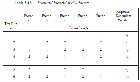
The “balance” referred to above, besides other aspects, can thus be noticed in the matrix.

1. In each column under the factors, there are as many level 1’s as there are level 2’s; this is also true for the entire matrix.
2. Except for the first line, which is used as the refer­ence for the “now” condition, all other lines have the same number of level 1’s (2) and level 2’s (3).

Using these values of dependent variables, shown only by the symbols y1 to y6 here, we can track the main effect of each factor, while acting in combination with other factors. The difference between the average of the values of dependent variables for a given factor when that factor is at level 2, and such an average when that factor is at level 1, is the measure of the main effect of that factor. For instance, the main effect of c is given by

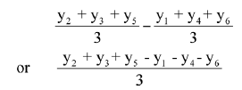
In the context of this experiment, if the above value is posi­tive, it indicates c as a beneficial factor. Similar values calculated for the other four factors will give us, on a comparative basis, the degree of effectiveness of all the factors. From these, we may identify the most effective one (or two) of the factors. For further optimization, one may plan for either a two-factor, two-level experiment or a two-factor, three-or-more-level experiment, as required. Tracing the interactions (not done here) between those two factors will then be fairly easy.

Source: Srinagesh K (2005), The Principles of Experimental Research, Butterworth-Heinemann; 1st edition.