Standard Normal Curve

The standard normal curve is, in fact, a generalization of many— as many as we may encounter—normal curves showing probabil­ity density distributions. Before we move to the generalization involved, it is relevant to examine the nature of the normal distri­bution curve. Firstly, it is not a frequency polygon, even if hun­dreds of straight lines are required to connect the points. Similarly, it is not a histogram, even if hundreds of “bars” consti­tute the figure, but the histogram may approximate the normal distribution curve, when the class widths are virtually reduced to lines. The normal distribution curve is, indeed, a continuous curve, bell-shaped and symmetrical about the mean of the vari­able. Though it is obtained purely as the outcome of a statistical procedure, it prevails as an embodiment of quantitative probabil­ity. It serves as a means, a tool, by which we can answer many questions of vital importance, such answers being the only ones possible in the absence of certainty. Based on such answers, deci­sions need to be made in daily business as well as in scientific inference. In way of preparing for the study of the standard nor­mal curve, let us make the following assumptions about data and procedures for obtaining the statistics on the height of adult males in, let us say, England.

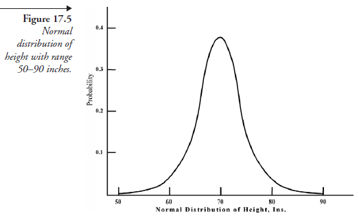
1. The range of heights is between 50 and 90 inches, and it was measured to a precision of 0.05 inch. Then, there are (90 – 50) ÷ 0.05 = 800 classes, each of 0.05 inch, for height as the variable.
2. The random sample consists of about ten thou­sand adult males.
3. A table of probability distribution, similar to Table 17.5 is prepared for the data

4. Using data from this table, a histogram of proba­bility density distribution, similar to Figure 17.3, is prepared.
5. Assuming that the class points at the top end of the bars conformed to a Gaussian distribution, which is very likely, a smooth curve is drawn.

The result then, in graphical form, will be as shown in Figure 17.5.

We note that the area under this curve (which is a measure of the sum of all probabilities) is of numerical value 1.0. Using this figure as the source, we may ask several probability questions.

1. What is the probability that the height of adult males of England will not exceed 63 inches? The answer to that question is given by the numerical value of the area under the curve up to sixty-three on the abscissa.
2. What is the probability that the height of adult males will exceed 75 inches? The answer to this question is given by the numerical value of the area under the curve beyond seventy-five on the abscissa.
3. What is the probability that the height of adult males will vary between 65 and 75 inches? The answer to this question is given by the numerical value of the area under the curve between sixty- five and seventy-five.

Each one of the above three questions, being only part of the area, is a fraction numerically less than one. In contrast, suppose we ask the question, What is the probability that the height of adult males in England will vary only between 50 and 90 inches? The answer is, obviously, the numerical value of the area under the curve between abscissas fifty and ninety. On impulse, we are likely to say it is 1.00, but reflecting on the nature of the normal distribution, we should say that it is very close to but less than 1.00. This is so because, at both ends, the normal distribution curve is asymptotic, extending from less than fifty to more than ninety and never touching the x-axis at either end.

Common to all four answers above is the phrase “numerical value of the area under the curve.” Obviously, the next important consideration is how to evaluate the area under the normal distri­bution curve. Here comes the well-known application of elemen­tary calculus. In the functional relation

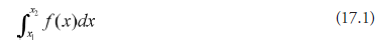
y takes different values as x varies over a range. If the different val­ues ofy, plotted as ordinates corresponding to the different values of x, when connected, form a smooth curve (or line), the area under the curve, corresponding to a range of x values, namely, between xi and xj, is obtained by integrating the function, f(x), between the limits xi and xj, symbolically expressed as

Now we recall that the normal distribution curve conforms to the functional relation:

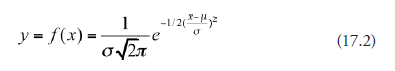
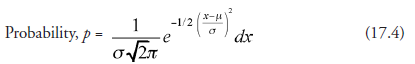
We have seen that in the graphical form of this relation (Fig­ure 17.5), the area under the curve between any two values of x is a measure of probability. Considering the interval on abscissa from x to (x + dx), we may now write the expression for probabil­ity corresponding to width dx as

 Substituting from (17.2), we get

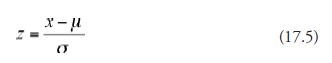
Suppose now that we adapt a new scale for measuring the range on the abscissa, with no other changes in the probability density curve, and this scale is related to x by

Then,

And in terms of z scale, the probability is given by

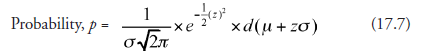
Considering that j and o are both constants for a given distri­bution, we get

Substituting (0 + o. dz) in place of d(j + zo) in (17.7), we get

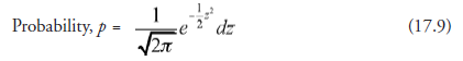
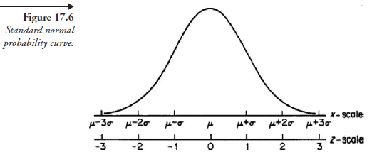
Comparing (17.9) with (17.4), we notice that (17.9) may be considered a particular case of (17.4), with fi = 0, o = 1, and z in place of x. This means that the graphical representation of (17.9) is a probability density curve. Such a curve is known as the stan­dard normal probability curve and is shown in Figure 17.7. It is the function of a random variable that has a normal distribution with a mean of 0 and a standard deviation of 1.0. We further note that any distribution of a random variable, so long as it is “normal,” can be reduced to this standard shape, represented by (17.9) by making the substitution as in (17.5); z then is known as the standard normal variable. And this entails that for a given normal distribution curve, the mean, fj,, and the standard devia-tion, O, of the random variable should be known before it can be rendered into this “standard” format.

For the purpose of illustrating the use of the standard normal distribution curve, we will ask questions pertaining to two diverse fields of interest:

1. Suppose the marketing department of a screw manufacturing company, on one of its products, a 1-inch screw, accepts the customer demand that screws either shorter than 97 inches or longer than 1.04 inches should be rejected. What is the probability that the company can meet this demand immediately without retooling?
2. What is the probability that the newborn babies in the United States have a length of only between 18 and 26 inches?

Question 1 above is from the area of quality control in man­ufacturing, and question 2 is from the area of health care. Sup­posing we have a normal distribution curve corresponding to question 1, we can get the answers in terms of the area under the curve, integrating (17.2), between appropriate limits as specified in the question. Depending on the probability density of the random variable, the shape of the curve corresponding to ques­tion 2 will be different from that for question 1. To answer any questions relative to this distribution, we need to perform another integration. Add to this that integration of this type of equations is not easy, though considerable help is now available from computers.

Suppose there is a need to integrate just one equation, and the results are applicable to any normal distribution whatsoever. That, precisely, is the equation that represents the standard nor­mal distribution. The integration is already done by the mathe­maticians; the area under the curve is evaluated for all possible limits to the required degree of accuracy and provided in the form of a compact table, referred to as “Areas of Probability for Standard Normal Distribution” (APSND). It is made available in many standard texts on statistics, as well as in books on other subjects having to deal with probability. It is reproduced here as Table 17.5.

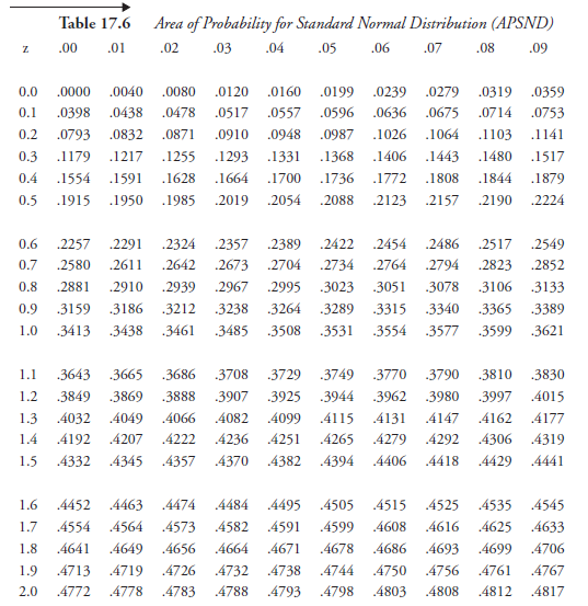
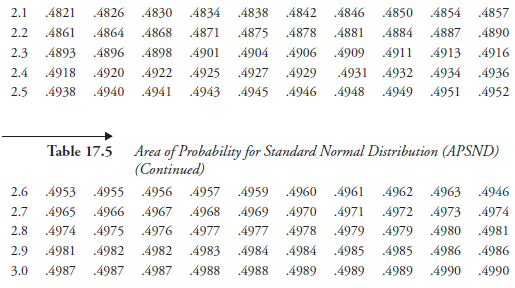
We need to develop familiarity with reading this table as a way of answering probability questions. The numerical value of z is read by combining the number in the left-hand column with the decimals of the top line. For example, z = 1.47 is obtained by 1.4 in the left-hand column, combined with 0.07 along the top line. Now, looking in the body of the table where the horizontal line of 1.4 meets the vertical column of 0.07, we find the number 0.4292. This is the area of the standard normal distribution between the mean (μ) and z = 1.47. It is the corresponding measure of probability, to be stated as, the probability that z varies between 0 and 1.47 is 0.4292. Thus, the area under the curve, between the mean (μ) and any specified positive value of z, can be read; the highest such value is 0.5.

Suppose we want to get probability corresponding to negative values of z. All we need to remember is that the normal distribution
curve is symmetrical, the shape of the curve to the left of the mean being a mirror image of the curve to the right of it. Conforming
to this, the area for the value z = –2.38, for instance, is 0.4913. And the probability value between z = –1.26 and z = +1.26 is given by (0.3962 + 0.3962) = 0.7924.

If we need to find the probability that z is higher than 2.45, we find the corresponding number in the table to be 0.4929.

Since 0.5 is the total area for z higher than the mean (μ), the area for z higher than 2.45 is (0.5 – 0.4929) = 0.0071; this is the measure of the corresponding probability.

Finally, suppose we need to find the probability that z is between 1.25 and 2.5. The area between z = 0 and z = 2.5 is 0.4938, and the area between z = 0 and z = 1.25 is 0.3944. Therefore, the area, the measure of probability required, is (0.4958 – 0.3944) = 0.1014.

Source: Srinagesh K (2005), The Principles of Experimental Research, Butterworth-Heinemann; 1st edition.