Theoretical Sampling Distribution of X

When we encounter finite but large or infinite populations, sam­pling is inevitable. Suppose we are interested in knowing the pop­ulation mean, the only connection we have with the population being the sample; we have to depend on the sample mean, which is not an exact but a “probabilistic” value, meaning it is reason­ably close to the population mean. Taking a sample from the population and finding the sample mean is, in effect, like doing an experiment with a given set of conditions. To increase the con­fidence in the experimental results, it is common to replicate the experiment; the greater the number of replications, the greater the confidence. If the experimental outcome, the dependent vari­able, is a number, then the number so obtained from several rep­lications will be averaged to get the “final” number as the experimental result. The equivalent in sampling is to get several
independent samples at random from the population, to find the mean from each sample, and then to get the mean of these means, a procedure that will increase the confidence (or the like­lihood) of the mean of the mean being close to the mean of the population.

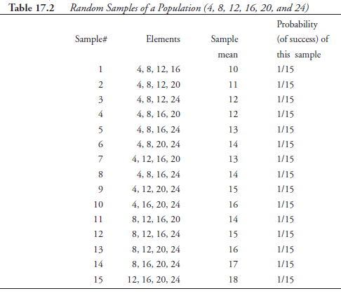
For demonstration purposes, we take a small population of only six elements: 4, 8, 12, 16, 20, and 24. If we decide, for instance, to draw four random samples from the population, those will be four out of all the possible combinations. The mean value of the four means, one from each sample, is then the prob­able mean of the population. By increasing the number of sam­ples, hence, the number of means to be averaged, we expect the probable mean to get even closer. With this in view, we will take all the possible samples, each of four elements, from the popula­tion, which is simply all the possible combinations of four ele­ments taken at a time, from a set of six elements. The number of such combinations is given by

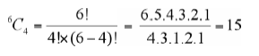
This means it is possible to draw fifteen different samples. The actual samples and their means are listed respectively in the second and the third columns of Table 17.2. Entries in the fourth column are to be interpreted as follows: When one of these fifteen possible samples is picked at random from the pop­ulation, the probability of success of this selection is 1/15, in the same way that the probability of success of getting a two from a throw of a die is 1/6, because there are six faces, each a possibil­ity, and two is the one that was successful in selection.

Now, if we take a close look at the third and the fourth col­umns of Table 17.2, we see another relation emerging. The mean value ten, with a probability of 1/15, appears in the list only once among the fifteen possibilities; the same is true for mean values eleven, seventeen, and eighteen. On the other hand, the mean value twelve is found twice, making the probability of its appear­ance 2 x 1/15 = 2/15; and the same is true for mean values thir­teen, fourteen, and fifteen. The mean value fourteen appears three times, making its probability 3 x 1/15 = 3/15. Extracting these facts from Table 17.2, a new relation between the value of the sample mean, X, and the corresponding probabilities (of suc-cess), designated as a probability function, fx), is shown in Table 17-3- Such relations as shown in this table are known as theoreti­cal sampling distribution for the population under consideration (finite or infinite).

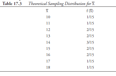
This relation is highly significant as we try to understand the nature of the population, with samples serving as the medium. The various statistical properties, both of the central tendency and the distribution, can be worked out reasonably closely through the data provided by theoretical sampling distribution. For instance, there are nine sample means in Table 17.3. The mean of the sample means is, thus, given by

We will separately calculate the mean of the population (which we happen to know entirely). It is given by:

This result is no coincidence. The truth of this “experiment” can be confirmed by considering much larger populations than the one of only six elements considered here. But the gravity of this significance is lost to us because not only do we know all the elements of the population, but also the population is small. If the population, instead, were very large (or infinite), like the height of all the tenth-grade boys in the United States, then to arrive at the mean height, we have to depend on sampling alone. Taking several samples and from those preparing a theoretical sampling distribution is the right procedure to follow. But it is to be noted that the particular statistic we so obtain, for instance, the mean of the population, can be only probabilistic, not exact as demonstrated above, which was made possible because in that case we knew the entire population.

In an infinite population, the number of samples that can be taken is also infinite; but practically, it is necessarily a finite, and often a limited, number. It can be intuitively understood that the larger the number of samples, and the larger the number of ele­ments in individual samples (these need not be the same from sample to sample), the closer the probable statistic to the corre­sponding one of the population. Summarized as follows are the procedural steps for preparing the theoretical sampling distribu-tion of sample means when the population is either too large to take all possible samples or it is simply infinite:

1. Take a random sample with a reasonably large number of elements; find the mean of this sample and call it X1.
2. As above, take a large number of independent, random samples, find the mean of each sample, and call these X2, X3, X4, . . . .
3. Out of such data, consisting of a conveniently large number of mean values, count the number of times X1 appeared and call this nx₁ also, find nx₂, ⁿX3, ⁿX4, . . . .
4. Find the numerical value of

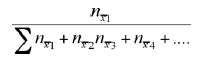
for all the data.

The above is a fraction expressing how frequently nx₁ appeared among all nx₂, nx₃, nx₄, . . . put together. It is known as the relative frequency of X1 we designate it as f(x1).

5. As above, find the relative frequencies of X2, X3 X4, . . .; designate these as f (x2), f (X3), f (X4), . . .
6. Then, prepare a table showing in two columns X1 versus f(X1), X2 versus f(x2), and so on, for all values of sampling means. This table is the theoretical sampling distribution of sample means for the population under consideration and is similar to Table 17.3.

In passing, we should note that the third column of Table 17.2 shows the mean, X, of each sample drawn. This is so because that is the particular statistic we chose to calculate for each sam­ple drawn. If we choose to calculate, instead, a different statistic, let us say the variance, we should have in that column a value for the variance of each sample. But the probability of each sample, shown in the fourth column of Table 17.2, would not have changed. Extracting data from such a table, we could have con­structed a theoretical sampling distribution for variance, as in Table 17.3, but with different numerical values in its two col­umns, namely, variance, s²_x, versus probability function of vari­ance, f(s²_x). In other words, it is possible to construct a theoretical sampling distribution of any statistic we choose, but statisticians prefer and rely more on the theoretical sampling dis­tribution of sample means than on any other statistic.

Using a theoretical sampling distribution of sample means as the source, it is possible to predict, that is, statistically calculate, other statistics of the population besides the population mean. It is to be understood that values so predicted have only probabilistic value, not certainty value. Even so, relations between predicted individual statistics of the population and the corresponding ones worked out using sample means are usually written in the form of equations. Though the empirical “truth” of these can be demon­strated by “experiments” using smaller populations, as was done before for population mean, we will skip that exercise and write the following relations:

μX = μx for all situations

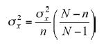
in which n is the number of elements in each of the many samples taken, when N is known

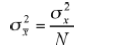
as above, but when N is infinite or very large

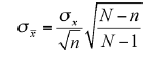
when N is known

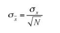
when N is infinite or very large

Revisiting Table 17.3, we need to make the following impor­tant observation. In the second column, we have various frac­tions: 1/15, 2/15, 3/15. The first one, 1/15, and the second one, 2/15, both appear four times, and the third one, 3/15, appears only once. Each of these represents the probability of success of the corresponding sample mean. Adding together all these prob­abilities, we get 4(1/15) + 4(2/15) + 1(3/15) = 1.0. This is anal­ogous to adding together the probabilities of rolling a one, two, three, four, five, and six, all the possibilities for a given dice throw; as each has a probability 1/6, adding them together yields 1.0. In a practical case of drawing many samples from a very large or infinite population, thereby constructing a theoretical sampling distribution of sample means, likewise we expect the sum of the probability functions to be close to, but not exceed, 1.0. That is,

Source: Srinagesh K (2005), The Principles of Experimental Research, Butterworth-Heinemann; 1st edition.