Money-Management Risks

We have defined risk in many ways in earlier chapters. Variability of returns, amount of loss per trade, beta, and maximum amount of loss per trade, drawdown, maximum drawdown, and volatility of prices have all been used. In Appendix A, we cover some of the statistical principles associated with risk measurement in Modern Portfolio Theory. One of the principal difficulties in the use of standard linear statistics in evaluating markets is that it assumes that each price, each trade, and each profit or loss is independent. In other words, it stands by itself and is not related to any other price, trade, or trade return. When using such statistics, one must, therefore, be careful not to believe absolutely in what the statistical tests might show.

1. Concepts

For our purposes, the important risk consideration is loss of capital. This comes from losses on trades, realized or unrealized, and, thus, we will use drawdowns as the best definition of risk. Because drawdowns, if not controlled, can lead to ruin, our intention in this chapter is to develop means that will keep us from losing all our capital.

2. Drawdown and Maximum Drawdown

When we discussed drawdowns in the previous chapter, we found that more than one drawdown can occur, and it may result from one trade or many trades. If we look at all the drawdowns over a period, the one that has the highest equity percentage loss is called the maximum drawdown (MDD). The MDD is the worst case that occurred in the system and often is used as an estimate of the worst case that can occur in the future. Of course, it could have been a fluke and exaggerate potential drawdowns in real trading, or it could underestimate and make drawdowns appear less damaging than they would be in real trading. We will find that we can reduce risk of loss on single trades with stops, but we cannot reduce the risk from a series of losses. All we can do is find a realistic estimate of the odds of a long run of losses against us and then take our chances or change the system. Even assuming a large MDD, we must design the money-management strategy such that enough capital is always available to withstand a loss in the magnitude of the known MDD. Otherwise, the system goes broke.

Drawdowns, for statistical purposes, are not independent, especially if the loss occurs in multiple systems at one time based on some adverse news. Uncontrollable loss, called an act of God in the insurance industry, or a Black Swan after the subject of the book by that name by Nassim Taleb (2010), cannot be anticipated and thus is never included in any estimate of risk. These events, however, usually only affect a single trade rather than a series of trades.

3. Theory of Runs

A drawdown is usually the result of a series of losses. We can estimate the chances of a series of losses using the theory of runs. This theory states that the probability of a series of independent events is the product of the probability of each event occurring. Thus, if a system has a losing percentage of 40%, the odds of a run of five losses in a row are (0.40 x 0.40 x 0.40 x 0.40 x 0.40) = .01 or 1%. If a system has a losing percentage of 60%, the odds of a run of five losses in a row are 8%. Although this calculation does not account for money lost in each transaction, it does suggest that to avoid a series of losses, the lower the losing percentage of the system, the better. Even so, a large number of losses together may not be harmful to a system specifically—many trend-following systems have long runs of losses—but create an additional risk of loss of confidence in the system and the potential premature abandonment just before it becomes profitable. Psychology is a major component in trading, and confidence is usually fragile when trades are going against the trader.

4. Martingale Betting System

A martingale betting system often is used in a situation where the bet size can be changed but the odds are relatively even, such as gambling at a roulette wheel. The basis for the method is the theory of runs and the odds against a long series of losses when probability is about even. The method is to double up on the next bet after a loss and return to the standard bet after a win. Eventually, a winning bet will cover all the previous losses and return a profit on the original bet. Unfortunately, the system requires substantial capital to withstand an unexpectedly long series of losses in a row.

For example, assume you make a $100 standard bet that takes the $100 bet and either returns the bet plus $100 on a win or pays nothing on a loss with even odds of winning or losing (50% win percentage). After a run of five successive losses occurs, using a martingale system, the next bet will require $3,200 above the $3,100 that has already been lost ($100 + $200 + $400 + $800 + $1,600 = $3,100). Thus, betting the sixth time after five successive losses would require $6,300, hoping for a win that would net $100 above our previous commitment. It is a tough way to make $100. Nevertheless, as long as the bettor can ante up the funds for the next bet in a losing series of bets, he will profit eventually by the amount of the original bet ($100) when the final winning bet occurs.

If the payoff ratio is greater than one-for-one and the win percentage is greater than 50%, the martingale approach may be profitable in the trading markets, but that long series of losses is always hanging out in space somewhere waiting to occur. Furthermore, in the trading markets, the profit from each bet is not constant. It could, for example, be larger for losses than for gains. Of course, a maximum loss or stop can be used to get out of the game, but by then so much capital has been lost that the chances of recovery are slim. Needless to say, the martingale approach rarely is used in trading markets.

5. Reward to Risk

The objective in all investment is to have a high reward to risk. Return on investment, or ROI, is the standard calculation of reward. ROI is calculated as net profit divided by initial capital at the beginning of the measured period. We have gone into more detail in Appendix A on statistics.

The standard method for analyzing portfolios and systems for reward and risk is to calculate the ratio of CAGR (compound annual growth rate) to the %MDD. This is called the MAR ratio and is how we initially evaluated the system design parameters in Chapter 22. Some analysts use other ratios. The profit/loss ratio, also called the profit factor, is commonly used, and the payoff ratio, which is the average gain per profitable trade to the average loss per unprofitable trade, is often used. Other methods of measuring specific aspects of a system or portfolio reward-to-risk are the Sharpe ratio, mentioned in Chapter 22 and Appendix A, and percent of winning trades.

A recent myth about MDD, derived from the risk-reward relationship in Modern Portfolio Theory, is that a higher MDD percent suggests a higher return. This is not true. Capital risk and reward are not proportional. MDD percent cannot be greater than 100%, but return can theoretically be infinite.

6. Normal Risks

The most important aspect of money management, beyond establishing where and what kind of stops to use to protect capital, is the determination of position size for each trade. Too much in a position can incur unwarranted risks in case of failure, including complete ruin, and too little can reduce profit potential beyond the risk-free rate. Position size is directly related to capital risk, the amount of money that can be lost, and it is the aspect of money management that most traders and investors overlook.

7. Position Size

By position size, we mean the amount of capital committed to a system or investment that incurs a specific risk. This is usually based on the difference between the entry price and exit price multiplied by the number of shares or contracts. As an example, let us assume we can only risk $500 in a trade. We have a breakout system that will buy a stock at $50. We place a protective sell stop at $45. This $5 difference in price is the capital risk we are taking per share. The entire position is not at risk because it will be liquidated on the stop. Without a stop, of course, we have no idea what risk we are taking. This is one reason fundamental analysis has trouble controlling capital risk. It has no means of determining when to exit a position. Knowing we have a $5 dollar per share risk, however, we know we can buy 100 shares for a total capital risk of our limit of $500.

In systems, position size has two levels of importance. The first is the determination of the minimum size of account required to trade a system with a minimum level of potential risk of ruin. The second is the determination of the optimal size of each position taken in a system that meets the predetermined risk level of the system owner. Generally, the position size in either determination is based on the maximum drawdown of the system and the margin required for a futures contract or price of a stock.

One problem does arise, and it has to do with short-term trading when the difference between prospective entry and exit price is small. This is best explained with an example. Say we have a $100,000 account and want to limit our losses to 2% of capital (that is, $2,000 per position). We find a $50 stock that we believe we can scalp for $2 with a risk of only $0.50. Using the risk formula and a 2% limit, we can buy 4,000 shares ($2,000 / $0.50 = 4,000). However, 4,000 shares of a $50 stock is $200,000, twice the amount of our capital. What do we do? We can borrow the extra $100,000 for the trade, but that leaves us with absolutely no room for another trade and exposes us to the risk of the debt. We can also cut back on the 4,000 shares to 2,000 shares, but by doing so we still haven’t freed enough capital for another trade and have cut our potential profit in half. To combat this problem, most traders use a smaller percent risk than 2% as their risk limit on a position. This makes sense not only for this situation, but because a scalper makes many trades a day, any one of which can go wrong, resulting in an increased risk of a long series of losses and a large drawdown. This method reduces that risk by limiting the potential trade loss to a smaller amount and allows more bad trades to occur without the risk of ruin.

8. Number of Shares or Contracts

In the stock market, the question of how many shares to use in a system is relatively easy because margin requirements are comparatively small and the number of shares flexible. In the futures markets, however, the number of contracts to use can become a problem. Margin requirements frequently change. The two standard methods of determining the number of contracts are either to use the system on a fixed number of contracts or to determine the risk as a percentage of the trading account and divide that by the margin required for each contract. After a successful series of trades, if the account capital has increased, a decision must be made as to whether to continue with a set number of contracts or continue with the percentage risk proportion on a continuous capital adjustment. Some traders use a capital step process whereby the number of contracts is only adjusted when the account capital reaches certain thresholds.

Evstigneev and Schenk-Hoppe (2001) argue that constant proportion strategies produce wealth more rapidly than other proportional methods. This is an outgrowth of the Kelly formula discussed next and implies that keeping a portfolio equally proportionally invested is the best method of accumulating profits. This concept goes against the grain of some analysts. They maintain that, although the system is working, the accumulation of profits is favorable. However, at some time, a significant series of losses will occur, when the capital is larger than its initial size. In that case, the losses will be proportionately larger because they depend on the proportion of the capital in the account. For now, we will go with the statistical evidence from Evstigneev and Schenk-Hoppe. They are not alone in their conclusions. As such, we will look for the optimal proportion of capital to invest in a system that will avoid the risk of total loss of capital. This sometimes is referred to as the fixed fractional method.

9. Determining Optimal Position Size

There are three methods of determining the position size: (1) risk of ruin formula, (2) theory of runs formula, and (3) optimal f or Kelly formula. To calculate the best position size, all three formulas should be used, and that formula with the smallest percentage of capital to be risked should be the one used in the system or model.

10. Risk of Ruin Formula

The risk of ruin (ROR) formula uses three pieces of data from the historical or testing data: (1) the probability of success or the percentage of wins; (2) the payoff ratio, or average win trade amount divided by the average loss trade amount; and (3) the fraction exposed to trading.

The risk of ruin formula (Kaufman, 1998) is

ROR = ((1 – ta) (1 + ta))^cu

Where:

ROR is the risk of ruin

ta is the trading advantage (percent wins minus percent losses)

cu is the number of trading units, shares, or contracts

Because the ratio is always less than one, the greater “cu” is, the less chance of ruin using a fixed dollar amount. In addition, the greater the “ta,” the less chance of ruin. The risk of ruin, therefore, is proportional to the percentage wins. The formula demonstrates that trend-following systems with a high percentage of losses often should end in ruin. This formula, however, fails to account for the amount of each win and loss.

To determine the optimal percentage of capital to use in any system with win and loss amounts, use this formula:

PCT = ([(A + 1) x p] – 1) / A

Where:

PCT is the percentage of capital to use

A is the average payoff ratio

p is the percentage of wins

Box 23.1 Optimal Percentage of Capital to Avoid Risk of Ruin

Using the figures from the example in Chapter 22, let us calculate the percentage of capital to use from the risk of ruin formula.

Data

(p) Percent profitable trades (profitable trades) = 64.71%

Average win trade amount = $929.07

Average loss trade amount = $393.42

(A) Average payoff ratio (average win/average loss) = 2.36

Formula

Optimal percentage of capital = {[(A + 1) x p] – 1} ÷ A

Substituting

Optimal percentage of capital = {[(2.36 + 1) x 0.6471] – 1} ÷ 2.36 = 49.8%

That is, any amount over 49.8% of capital in this system has a high chance of ending in ruin.

The high percentage suggests that the risk of ruin is low for normal commitments of 2%.

11. Theory of Runs

The chance of going broke from a series of losses is the amount of trading times the percentage of losses to the power of the largest string of losses. Most analysts will assume a minimum run of ten consecutive losses as the baseline. In any case, most calculations end with a maximum suggested percentage investment of around 2% to avoid the risk of going broke.

12. Optimal fand the Kelly Formula

The Kelly formula was invented by John L. Kelly, Jr. of Bell Labs in the early 1940s to measure long­distance telephone noise and was later adopted by gamblers to determine optimal betting sizes. Its application to the trading markets is somewhat tenuous because it does not account for MDD and, thus, risk of ruin. However, it is used in conjunction with other position-size calculations to determine the optimal size of a position relative to capital. In any profitable system, capital growth increases in proportion to the percentage of capital risked. After a certain threshold in the percentage, however, the rate of growth decreases and eventually reaches zero. The Kelly ratio or optimal f is the threshold of maximum growth. Optimal f is, therefore, a method of determining the optimal percentage of capital that should be invested in a particular system.

The optimal f percentage = (percentage of wins x (profit factor + 1) – 1) / profit factor Where: Percentage of wins is the percentage of winning trades Profit factor is the ratio of total gains over total losses

Once f is determined, it is multiplied times capital for the amount to be used in each position. This amount can be divided by the contract margin requirement for each contract to determine the number of contracts. In the stock market, the amount for each position can be divided by the price of the shares to determine the number of shares. Because this method often suffers from extraordinary drawdowns, the percentage of capital is usually limited to 0.8 of optimal f, or a maximum optimal f of 25%.

To account for MDD that is otherwise not in the f formula, another method called secure f (Zamansky and Stedhahl, 1998) is to divide the MDD by optimal f to determine the amount that can be risked on one contract or convert this amount to a percentage of capital for stock shares. The Larry Williams formula for the number of contracts to trade is to take the amount of money at risk (account balance times risk percent from whatever formula) divided by the largest single loss. A loss in the future can be controlled by stops.

Box 23.2 Calculating Optimal F Again, using the system developed in Chapter 22, let us calculate the optimal f.

Formula

Optimal f = (percentage of wins x (profit factor + 1) – 1) / profit factor

Data

Percentage of wins =64.71%

Profit factor            =4.33

S ubstituting

Optimal f                 = (.6471; x (4.33 + 1) – 1) / 4.33

                                = 56.6%

This is the maximum percentage to invest any capital account in the HAL system developed in Chapter 22.

13. Final Position Size

The smallest percentage of capital suggested by the three formulas is used as the final percentage for trading the specified system. Generally, because the theory of runs limits the percentage to around 2%, most professional traders use this figure, or less, as a maximum commitment to any system. In the HAL system, however, the percentage of losses is so small that the odds of a run of five losses is almost negligible. Thus, the other methods should take precedence, and each shows that a substantial portion of assets could have been invested in the system.

14. Initial Capital

The reason for concern about initial capital requirements is the risk of a series of losses right in the beginning of the system use. The problem at start-up is not the problem of individual loss in a trade. That can be controlled with stops. The problem is the risk of complete loss of capital. This problem is related to the possibility of a run of losses that wipes out capital and eliminates the trader from being able to reenter the system. Later, when profits have accrued, the accumulated profit cushion lessens the risk of losing all, but at the start, the risk of being wiped out is the highest.

A general rule of thumb for initial capital is to have at least three times the margin required for a single contract for each contract traded, or at least two times the amount of the MDD plus the initial margin for stocks and contracts. A more precise number can be determined from the Monte Carlo simulation described previously, estimating the odds of complete failure of the system using history. As in any simulation, the levels determined from the test should be doubled or tripled as a precaution against extraordinary initial surprises.

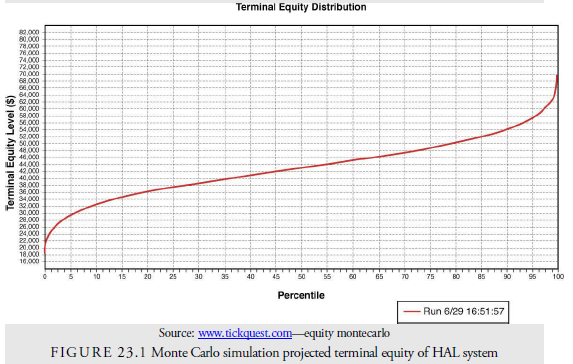
Box 23.3 Initial Capital—Monte Carlo Simulation

In Chapter 22, we developed the HAL trading system. Now, using a Monte Carlo simulation of the HAL system, let us look at a chart of the distribution of terminal equity for the total number of tests. The test period was nine years, seven months, and five days, and 300 positions were taken for an average of 46 per year. The initial price of IBM was $88.02, and we assume all trades are 100 shares. We set original capital at $30,000 and the maintenance capital at $1,000. This is the level below which our system goes broke. (We need the remaining $1,000 to close up shop and go home.) We then run the simulation to see if the system can withstand a series of adverse runs within a year.

The lower line in Figure 23.1 shows the results for an initial capital of $30,000. At the 50% vertical line, the upper line appears at $43,000. This means that 50% of the upper tests beginning with $30,000 had ending equity of $43,000 or less. At no time in the 3,000 simulations did the HAL go broke within the first year.

15. Leverage

Leverage, or the borrowing of capital to increase the potential for gain, of course, also increases the risk. Leverage generally increases the volatility of the portfolio or system and, thus, magnifies all those dangerous possibilities from increased volatility, including larger drawdowns and more potential for complete failure.

Risk is proportional to leverage. If we find that our system or combination of systems produces an MDD that is unacceptably high, we can adjust the portfolio mix to include a risk-free investment, such as Treasury bills, in the proportion necessary to bring down the potential MDD. For example, if the model estimates a 40% MDD, and we will accept only a 20% MDD, we can adjust the model to invest 50% of the capital in risk-free investments and the remainder in the systems. On the other hand, if the systems suggest a 10% MDD, and we are willing to accept a 20% MDD, we can borrow 100% of the model’s capital and double our return as well as our risk.

16. Pyramiding

Pyramiding is a more complicated method of adding leverage to a position. It consists of adding to a profitable position to gain leverage. Of course, the risks are not as clear because gaining size in the position after it is profitable may result in a larger position just as the inevitable drawdown begins. The best manner of pyramiding is to test it within the system as a set of rules. Specific rules of thumb for pyramiding include the following:

1. Never adding to a position until its profit becomes positive
2. Placing stops at the break-even level as size increases
3. Entering the largest positions first and diminishing the size of subsequent entries
4. Being sure that the position risk is still within the limits established by the system and by the maximum acceptable position size

17. Unusual Risks

Before we become involved in standard portfolio risks, we must be aware of other risks that we have some control over but that will not usually show up in standard tests of performance. These are outlined next.

18. Psychological Risk

As we have mentioned many times earlier, trading and investing are largely psychological. The motion of investment vehicles is due largely to rational and to irrational decisions on the part of buyers and sellers. Taking advantage of this price motion through technical analysis is an emotional exercise for the trader or investor as well. The participant in the markets must be careful not to be swept up in the emotion of the crowd; indeed, in many instances, she must act against the crowd and, thus, against human nature. Many inputs can affect the psychological stability of the trader. Lack of sleep, family fight, sickness, or any other nonstandard outside intervention can upset one’s attitude and ability to act successfully. Unfortunately, once lack of success begins, lack of confidence also begins, and lack of confidence can cause even more errors in judgment. The purpose in designing a nondiscretionary system is to reduce those outside emotional effects and let the system operate by itself. However, a losing system or series of losses can cause even the slightest override of the system; simply a change in orders, a wait after a breakout, or any other minor action unknowingly can upset the expected results even more. Many system overrides are not even recognized by the trader—just a little change here and there. Thus, there is a constant battle between the psyche and the markets. A supersystem will not avoid one’s own nature. Only one can control one’s nature. It is a risk that cannot be eliminated by a computer—only reduced —and the system must be followed religiously. Some writers argue that the psychology of trading accounts for better than 70% of success. This is likely true, but unfortunately, it is perverse and unquantifiable.

19. Knowledge of the Market

“I didn’t realize that option expired today” or “I didn’t realize that contract traded at night in Singapore” can be costly mistakes. The trader or investor must be fully aware of the markets being traded, their history, their method of execution, their various peculiarities, their people, their structure, and their operation. There is no excuse for losing money from simple ignorance. Most investors learn from experience about the oddities of particular markets, but that experience can be costly.

20. Diversifiable Risk

Diversification is a complex subject. As we saw in Chapter 22, the complexity has to do with the weighting amount of different vehicles or systems in a portfolio, as well as whether the behaviors of the components are similar or different from each other. Various mathematical models have been developed; but as we said before, diversification is the commonsense approach of “not putting all your eggs in one basket” that is needed. Obviously, if different vehicles or systems are used, they should not act in concert. Otherwise, they are essentially the same system, and risk has not been diversified away.

Risk is both correlated and uncorrelated. Correlated risk cannot be eliminated through diversification. We must use other means. This nondiversifiable, or market, risk is the risk generated by the overall market itself and accounts for a large portion of portfolio risk. Uncorrelated risk, however, can be reduced through diversification. Uncorrelated risk comes from the effects of all sorts of exogenous variables on individual issues and has more to do with the risk of the individual issue than the overall market. Uncorrelated risk can be reduced by diversification into dissimilar or uncorrelated issues or systems.

An example of correlated, nondiversifiable risk would be the risk that the Federal Reserve tightening the money supply will have a widespread impact on security values and affect almost any stock in a portfolio. On the other hand, the risk that a Vioxx lawsuit will decrease the value of Merck stock is uncorrelated, diversifiable risk. The lawsuit would not impact the stocks of other companies.

Reduction in uncorrelated risk can reduce MDD and enhance ROI. Indeed, the results of a diversified portfolio are often superior to the results from the best individual system by itself. The Capital Asset Pricing Model suggests that a properly structured 9-stock portfolio reduces the uncorrelated risk to that of one-third the risk of a single stock. A 16-stock portfolio can reduce uncorrelated risk to one-fourth that of a single stock. The relationship is based on the inverse square root of the number of stocks in the portfolio. As such, the portfolio can never eliminate uncorrelated risk, but with just a few different issues or systems, it can reduce it enough to make it irrelevant. The real problem then becomes the effect of correlated risk as in the debt crisis in 2008-2009 when many investments that had earlier been uncorrelated suddenly became correlated and declined together. What constitutes correlation in investments or systems, then, is a subject equally difficult to assess. Some investors believe that diversification detracts from performance because it dilutes reward along with risk. Using specific selection methods to concentrate on the investments with the most potential, they use exit strategies in individual issues to reduce uncorrelated risk and market timing for the entire portfolio to reduce correlated risk. (For more details on the mathematics behind diversification and portfolio theory, refer to Appendix A.)

One further complication in the subject of correlations is that often a lead-lag relationship occurs that is invisible to the system tester, and most correlations themselves change over time. Efficient diversification is, thus, a useful and important subject but not a simple one.

21. Trade Frequency

Ten losing trades in different markets is the same as ten consecutive losses in one market. The drawdown is the same. Thus, diversification can bring problems as well as reduce risk. The frequency of trading in different markets will increase the risk of a series of losses across markets.

22. Temporal

Risk increases with time. The longer a position is held, the more risky it becomes. This is why long-term interest rates are usually higher than short-term rates. On the other hand, in the markets, reward does not increase with time. Thus, to reduce risk, a position should not be held beyond the time that reward ends. Then, only risk remains.

23. Security Quality

If given the choice of trading a high-quality issue (as determined by some financial rating service) that has the same market characteristics as a low-quality issue, including volatility, liquidity, and volume, which would you choose? The high-quality issue, of course. Erroneously, quality is a concept that normally is not addressed and certainly is not a factor in most systems models.

Source: Kirkpatrick II Charles D., Dahlquist Julie R. (2015), Technical Analysis: The Complete Resource for Financial Market Technicians, FT Press; 3rd edition.