Estimating and Predicting Cost of Production

A business that is expanding or contracting its operation must predict how costs will change as output changes. Estimates of future costs can be obtained from a cost function, which relates the cost of production to the level of output and other variables that the firm can control.

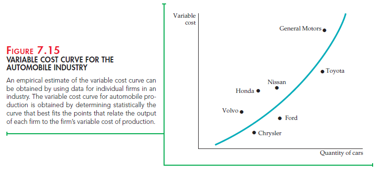
Suppose we wanted to characterize the short-run cost of production in the automobile industry. We could obtain data on the number of automo- biles Q produced by each car company and relate this information to the company’s variable cost of production VC. The use of variable cost, rather than total cost, avoids the problem of trying to allocate the fixed cost of a multiproduct firm’s production process to the particular product being studied.16

Figure 7.15 shows a typical pattern of cost and output data. Each point on the graph relates the output of an auto company to that company’s variable cost of production. To predict cost accurately, we must determine the underlying relationship between variable cost and output. Then, if a company expands its production, we can calculate what the associated cost is likely to be. The curve in the figure is drawn with this in mind—it provides a reasonably close fit to the cost data. (Typically, least-squares regression analysis would be used to fit the curve to the data.) But what shape is the most appropriate, and how do we represent that shape algebraically?

Here is one cost function that we might choose:

VC = bq                                             (7.9)

Although easy to use, this linear relationship between cost and output is applicable only if marginal cost is constant.^[1] For every unit increase in output, variable cost increases by b; marginal cost is thus constant and equal to b-

If we wish to allow for a U-shaped average cost curve and a marginal cost that is not constant, we must use a more complex cost function. One possibility is the quadratic cost function, which relates variable cost to output and output squared:

vc = bq + gq²                                          (7.10)

This function implies a straight-line marginal cost curve of the form MC = b + 2g q.¹⁸ Marginal cost increases with output if g is positive and decreases with output if g is negative.

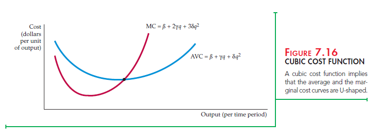
If the marginal cost curve is not linear, we might use a cubic cost function:

vc = bq + gq² + dq³                                       (7.11)

Figure 7.16 shows this cubic cost function. It implies U-shaped marginal as well as average cost curves.

Cost functions can be difficult to measure for several reasons. First, output data often represent an aggregate of different types of products. The automo­biles produced by General Motors, for example, involve different models of cars. Second, cost data are often obtained directly from accounting information that fails to reflect opportunity costs. Third, allocating maintenance and other plant costs to a particular product is difficult when the firm is a conglomerate that produces more than one product line.

Cost Functions and the Measurement of Scale Economies

Recall that the cost-output elasticity E_C is less than one when there are econo­mies of scale and greater than one when there are diseconomies of scale. The scale economies index (SCI) provides an index of whether or not there are scale economies. SCI is defined as follows:

SCI = 1 – E_C                                           (7.12)

When E_C = 1, SCI = 0 and there are no economies or diseconomies of scale. When E_C is greater than one, SCI is negative and there are diseconomies of scale. Finally, when E_C is less than 1, SCI is positive and there are economies of scale.

Source: Pindyck Robert, Rubinfeld Daniel (2012), Microeconomics, Pearson, 8th edition.