Trade-Offs in Supply Chain Transportation Design

All transportation decisions made by shippers in a supply chain network must take into account their impact on inventory costs, facility and processing costs, the cost of coordinating operations, and the level of responsiveness provided to customers. For example, Amazon’s use of package carriers to deliver products to customers increases transportation cost but allows Amazon to cen­tralize its facilities and reduce inventory costs. If Amazon wants to reduce its transportation costs, the company must either sacrifice responsiveness to customers or increase the number of facilities and resulting inventories to move closer to customers.

The cost of coordinating operations is generally hard to quantify. Shippers should evaluate different transportation options in terms of various costs and revenues and then rank them accord­ing to coordination complexity. A manager can then make the appropriate transportation deci­sion. Managers must consider the following trade-offs when making transportation decisions:

• Transportation and inventory cost trade-off
• Transportation cost and customer responsiveness trade-off

1. Transportation and inventory Cost Trade-Off

The trade-off between transportation and inventory costs is significant when designing a supply chain network. Two fundamental supply chain decisions involving this trade-off are

• Choice of transportation mode
• Inventory aggregation

CHOICE OF TRANSPORTATION mode Selecting a transportation mode is both a planning and an operational decision in a supply chain. The decision regarding carriers with which a company contracts is a planning decision, whereas the choice of transportation mode for a particular ship­ment is an operational decision. For both decisions, a shipper must balance transportation and inventory costs. The mode of transportation that results in the lowest transportation cost does not necessarily lower total costs for a supply chain. Cheaper modes of transport typically have longer lead times and larger minimum shipment quantities, both of which result in higher levels of inventory in the supply chain. Modes that allow for shipping in small quantities lower inventory levels but tend to be more expensive. Apple, for example, airfreights several of its products from Asia. This choice cannot be justified on the basis of transportation cost alone. It can be justified only because the use of a faster mode of transportation for shipping valuable components allows Apple to carry low levels of inventory and still be responsive to its customers.

The impact of using different modes of transportation on inventories, response time, and costs in the supply chain is shown in Table 14-3. Each transportation mode is ranked along vari­ous dimensions, with 1 being the best and 6 being the worst.

Faster modes of transportation are preferred for products with a high value-to-weight ratio (an iPad is a good example of such a product) for which reducing inventories is important, whereas cheaper modes are preferred for products with a small value-to-weight ratio (e.g., fur­niture imported by IKEA) for which reducing transportation cost is important. The choice of transportation mode should take into account potential lost sales and cycle, safety, and in-transit inventory costs in addition to the cost of transportation. The lost sales and inventory costs are influenced by the speed, flexibility, and reliability of the mode. The purchase price must also be included if it changes with the choice of transportation mode (perhaps because of a change in lot sizes). Ignoring inventory costs when making transportation decisions can result in choices that worsen the performance of a supply chain, as illustrated in Example 14-2 (see worksheet Example14-2).

EXAMPLE 14-2 Trade-Offs When Selecting Transportation Mode

Eastern Electric (EE) is a major appliance manufacturer with a large plant in the Chicago area. EE purchases all the motors for its appliances from Westview Motors, located near Dallas. EE currently purchases 120,000 motors each year from Westview at a price of $120 per motor. Demand has been relatively constant for several years and is expected to stay that way. Each motor averages about 10 pounds in weight, and EE has traditionally purchased lots of 3,000 motors. Westview ships each EE order within a day of receiving it (lead time is one day more than transit time). At its assembly plant, EE carries a safety inventory equal to 50 percent of the average demand for motors during the replenishment lead time.

The plant manager at EE has received several proposals for transportation and must decide on the one to accept. The details of various proposals are provided in Table 14-4, where one cwt equals 100 pounds.

Golden’s pricing represents a marginal unit quantity discount (see Chapter 11). Golden’s representative has proposed lowering the marginal rate for the quantity over 250 cwt in a ship­ment from $4/cwt to $3/cwt and suggested that EE increase its batch size to 4,000 motors to take advantage of the lower transportation cost. What should the plant manager do?

Analysis:

Golden’s new proposal will result in low transportation costs for EE if the plant manager orders in lots of 4,000 motors. The plant manager, however, decides to include inventory costs in the transportation decision. EE’s annual cost of holding inventory is 25 percent, which implies an annual holding cost of H = $120 X 0.25 = $30 per motor. Shipments by rail require a five-day transit time, whereas shipments by truck have a transit time of three days. The transportation decision affects the cycle inventory, safety inventory, and in-transit inventory for EE. Therefore, the plant manager decides to evaluate the total transportation and inventory cost for each trans­portation option.

The AM Rail proposal requires a minimum shipment of 20,000 pounds or 2,000 motors. The replenishment lead time in this case is L = 5 + 1 = 6 days. For a lot size of Q = 2,000 motors, the plant manager obtains the following:

Cycle inventory = Q/ 2 = 2,000 /2 = 1,000 motors

Safety inventory = L/ 2 days of demand = (6 / 2)( 120,000 /365) = 986 motors

In-transit inventory = 120,000(5 / 365) = 1,644 motors

Total average inventory = 1,000 + 986 + 1,644 = 3,630 motors

Annual holding cost using AM Rail = 3,630 X $30 = $108,900

AM Rail charges $6.50 per cwt, resulting in a transportation cost of $0.65 per motor because each motor weighs 10 pounds. Here we have approximated the holding cost because we have not included the transportation cost in the cost of the product. A more precise evaluation would set the holding cost of in-transit inventory to be $30 (because transportation cost has not yet been incurred) and the holding cost of cycle and safety inventory to be 120.65 X 0.25 = $30.16 because transportation cost has been incurred by this stage. The precise evaluation would result in an inventory holding cost of (1,644 X 30) + (1,986 X 30.16) = $109,218.

The annual transportation cost is obtained as follows:

Annual transportation cost using AM Rail = 120,000 X 0.65 = $78,000

The total annual cost for inventory and transportation using AM Rail is thus $186,900.

The plant manager then evaluates the cost associated with each transportation option, as shown in Table 14-5 (we have used the approximate inventory cost in this analysis, applying the holding cost only to the unit cost and not the unit cost plus transportation cost/unit). (See work­sheet Example14-2 for all details in Table 14-5.) Based on the analysis in Table 14-5 (the inven­tory numbers are rounded to the closest integer), the plant manager decides to sign a contract with Golden Freightways and order motors in lots of 500. This option has the highest transporta­tion cost, but the lowest overall cost. If the selection of the transportation option were made using only the transportation cost incurred, Golden’s new proposal lowering the price for large ship­ments would look attractive. In reality, though, EE pays a high overall cost for this proposal because of the high inventory costs that result. Thus, considering the trade-off between inventory and transportation costs allows the plant manager to make a transportation decision that mini­mizes EE’s total cost.

Key Point

When selecting a mode of transportation, managers must account for unit costs and cycle, safety, and in-transit inventory costs that result from using each mode. Modes with high transportation costs can be justified if they result in significantly lower inventory costs.

INVENTORY AGGREGATION Firms can significantly reduce the safety inventory they require by physically aggregating inventories in one location (see Chapter 12). Most online businesses use this technique to gain advantage over firms with facilities in many locations. For example, Amazon has focused on decreasing its facility and inventory costs by holding inventory in a few warehouses, whereas booksellers such as Barnes & Noble must hold inventory in many retail stores.

Transportation cost, however, generally increases when inventory is aggregated. If inventories are highly disaggregated, some aggregation can also lower transportation costs. Beyond a certain point, though, aggregation of inventories raises total transportation costs. Consider a bookstore chain such as Barnes & Noble. The inbound transportation cost to Barnes & Noble is due to the replenishment of bookstores with new books. There is no outbound cost because customers transport their own books home. If Barnes & Noble decides to close all its bookstores and sell only online, it will have to incur both inbound and outbound transportation costs. The inbound transportation cost to warehouses will be lower than to all bookstores. On the outbound side, however, transportation cost will increase significantly because the out­bound shipment to each customer will be small and will require an expensive mode such as a package carrier. The total transportation cost will increase on aggregation because each book travels the same distance as when it was sold through a bookstore, except that a large fraction of the distance is on the outbound side using an expensive mode of transportation. As the degree of inventory aggregation increases, total transportation cost goes up. Another compari­son is in the video rental business between Netflix and Redbox. Netflix aggregates its invento­ries, thus lowering facility and inventory expense. It does, however, have to pay to ship DVDs between its DCs and customer homes. Redbox, in contrast, has many vending machines that carry DVDs but incurs low transportation costs. Thus, all firms planning inventory aggregation must consider the trade-offs among transportation, inventory, and facility costs when making this decision.

Inventory aggregation is a good idea when inventory and facility costs form a large fraction of a supply chain’s total costs. Inventory aggregation is useful for products with a large value-to- weight ratio and for products with high demand uncertainty. For example, inventory aggregation is valuable in the diamond industry, because diamonds have a large value-to-weight ratio and demand is uncertain. Inventory aggregation is also a good idea if customer orders are large enough to ensure sufficient economies of scale on outbound transportation. When products have a low value-to-weight ratio and customer orders are small, however, inventory aggregation may hurt a supply chain’s performance because of high transportation costs. Compared with dia­monds, the value of inventory aggregation is smaller for best-selling books that have a lower value-to-weight ratio and more predictable demand.

We illustrate the trade-off involved in making aggregation decisions in Example 14-3 (see worksheet Example14-3).

EXAMPLE 14-3 Trade-Offs When Aggregating Inventory

HighMed, a manufacturer of medical equipment used in heart procedures, is located in Madison, Wisconsin. Cardiologists use its products all over North America. The medical equipment is sold not through purchasing agents, but rather directly to doctors. HighMed currently divides the United States into twenty-four territories, each with its own sales force. All product inventories are maintained locally and replenished from Madison every four weeks using UPS. The average replenishment lead time using UPS is one week. UPS charges at a rate of $0.66 + 0.26x, where x is the quantity shipped in pounds. The products sold fall into two categories—HighVal and LowVal. HighVal products weigh 0.1 pounds and cost $200 each. LowVal products weigh 0.04 pounds and cost $30 each.

Weekly demand for HighVal products in each territory is normally distributed, with a mean of = 2 and a standard deviation of s_H = 5. Weekly demand for LowVal products in each territory is normally distributed, with a mean of m_L = 20 and a standard deviation of s_L = 5. HighMed maintains sufficient safety inventories in each territory to provide a CSL of 0.997 for each product. Holding cost at HighMed is 25 percent.

In addition to the current approach, the management team at HighMed is considering two other options:

Option A: Keep the current structure but replenish inventory once a week rather than once every four weeks.

Option B: Eliminate inventories in the territories, aggregate all inventories in a finished- goods warehouse at Madison, and replenish the warehouse once a week.

If inventories are aggregated at Madison, orders will be shipped using FedEx, which charges $5.53 + 0.53x per shipment, where x is the quantity shipped in pounds. The factory requires a one-week lead time to replenish finished-goods inventories at the Madison warehouse. An average customer order is for 1 unit of HighVal and 10 units of LowVal. What should HighMed do?

Analysis:

HighMed can reduce transportation cost by aggregating the quantity shipped at a time because prices for both UPS and FedEx display economies of scale. When comparing Option A with the current system, the management team must trade off the savings in transportation cost through less frequent replenishment with the savings in inventory cost with more frequent replenishment. When considering Option B, the management team must trade off the increase in transportation cost upon aggregation of inventories and the use of a faster but more expensive carrier (FedEx) with the decrease in inventory cost.

The management team first analyzes the current situation. For each territory,

Replenishment lead time, L = 1 week

Reorder interval, T = 4 weeks

CSL = 0.997

1. HighMed inventory costs (current scenario): For HighVal in each territory, the man­agement team obtains the following:

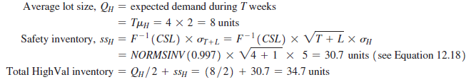
Across all twenty-four territories, HighMed thus carries HighVal inventory of 24 X 34.7 = 832.8 units (the true number is 833.3 units if we do not round inventory values to the first decimal). For LowVal in each territory, the management team obtains the following:

Across all 24 territories, HighMed thus carries LowVal inventory = 24 X 70.7 = 1696.8 units (the true number is 1697.3 if we do not round safety inventory to the first decimal).

The management team thus obtains the following:

Annual inventory holding cost for HighMed = (average HighVal inventory X $200 + average LowVal inventory X $30) X 0.25

= (832.8 X $200 + 1696.8 X $30) X 0.25

= $54,366 ( $54,395 without rounding)

2. HighMed transportation cost (current scenario):The average replenishment order from each territory consists of Q_H = 8 units of HighVal and Q_L = 80 units of LowVal. Thus, Average weight of each replenishment order

= 0.1 Q_h + 0.04Q_l = 0.1 X 8 + 0.04 X 80 = 4 pounds

Shipping cost per replenishment order = $0.66 + 0.26 X 4 = $1.70

Each territory has 13 replenishment orders per year and there are 24 territories.

Thus, Annual transportation cost = $1.70 X 13 X 24 = $530

3. HighMed total cost (current scenario): Annual inventory and transportation cost at

HighMed = inventory cost + transportation cost = $54,366 + $530 = $54,896 ($54,926 without rounding).

The HighMed management team evaluates the costs for Option A and Option B similarly; the results are summarized in Table 14-6. The results in Table 14-6 are reported without rounding and can be obtained from the associated worksheet Example14-3.

From Table 14-6, observe that increasing the replenishment frequency under Option A decreases total cost at HighMed. The increase in transportation cost is much smaller than the decrease in inventory cost resulting from smaller lots. HighMed is able to reduce total cost most by aggregating all inventories and using FedEx for transportation, because the decrease in inventories upon aggregation is larger than the increase in transportation cost.

The value of aggregation is affected by transportation cost, uncertainty of demand, holding cost, and the size of customer orders. If transportation costs were to double for HighMed, the decentralized Option A would become cheaper than the centralized Option B (in this setting, Option A costs $32,109, whereas Option B costs $37,402). As transportation cost increases, it becomes cheaper to decentralize inventories even though inventory costs increase.

If demand uncertainty decreases (e.g., the standard deviation of weekly demand for HighVal decreases from 5 to 2), the decentralized Option A would again become cheaper than the centralized Option B. As demand uncertainty decreases, it becomes cheaper to decentralize inventories.

If holding cost decreases (e.g., the holding cost drops to 12.5 percent from 25 percent), the decentralized Option A would again become cheaper than the centralized Option B. As product value or holding cost decreases, it becomes cheaper to decentralize inventories.

If customer order sizes are small, the increase in transportation cost upon aggregation can be significant, and inventory aggregation may increase total costs. Reconsider the case of HighMed, but now each customer order averages 0.5 HighVal and 5 LowVal (half the size con­sidered earlier). The costs for the current option as well as Option A remain unchanged because HighMed does not pay for outbound transportation and incurs only the cost of transporting replenishment orders under both options. Option B, however, becomes more expensive because outbound transportation costs increase with a decrease in customer order size. With smaller cus­tomer orders, the costs under Option B are as follows:

Average weight of each customer order = 0.1 X 0.5 + 0.04 X 5 = 0.25 pounds

Shipping cost per customer order = $5.53 + 0.53 X 0.25 = $5.66

Number of customer orders per territory per week = 4

Total customer orders per year = 4 X 24 X 52 = 4,992

Annual transportation cost = 4,992 X $5.66 = $28,255 ($28,267 without rounding)

Total annual cost = inventory cost + transportation cost = $8,474 + $28,255 = $36,729 ($36,740 without rounding)

Thus, with small customer orders, inventory aggregation is no longer the lowest-cost option for HighMed because of the large increase in transportation costs. The company is better off maintaining inventory in each territory and using Option A, which gives a lower total cost.

The lessons from Example 14-3 (and Chapter 12) with regard to inventory aggregation are summarized in Table 14-7.

2. Trade-Off Between Transportation Cost and Customer Responsiveness

The transportation cost a supply chain incurs is closely linked to the degree of responsiveness the supply chain aims to provide. If a firm has high responsiveness and ships all orders within a day of receipt from the customer, it will have small outbound shipments, resulting in a high transpor­tation cost. If it decreases its responsiveness and aggregates orders over a longer time horizon before shipping them out, it will be able to exploit economies of scale and incur a lower transpor­tation cost because of larger shipments. Temporal aggregation is the process of combining orders across time. Temporal aggregation decreases a firm’s responsiveness because of shipping delay, but also decreases transportation costs because of economies of scale that result from larger ship­ments. Thus, a firm must consider the trade-off between responsiveness and transportation cost when designing its transportation network, as illustrated in Example 14-4.

EXAMPLE 14-4 Trade-Off Between Transportation Cost and Responsiveness

Alloy Steel is a steel service center in the Cleveland area. All orders are shipped to customers using an LTL carrier that charges $100 + 0.01x, where x is the number of pounds of steel shipped on the truck. Currently, Alloy Steel ships orders on the day they are received. Allowing for two days in transit, this policy allows Alloy to achieve a response time of two days. Daily demand at Alloy Steel over a two-week period is shown in Table 14-8.

The general manager at Alloy Steel believes that customers do not really value the two-day response time and would be satisfied with a four-day response. What are the cost advantages of increasing the response time?

Analysis:

As the response time increases, Alloy Steel has the opportunity to aggregate demand over mul­tiple days for shipping. For a response time of three days, Alloy Steel can aggregate demand over two successive days before shipping. For a response time of four days, Alloy Steel can aggregate demand over three days before shipping. The manager evaluates the quantity shipped and trans­portation costs for different response times over the two-week period, as shown in Table 14-9 (see worksheet Example14-4).

From Table 14-9, observe that the transportation cost for Alloy Steel decreases as the response time increases. The benefit of temporal consolidation, however, diminishes rapidly upon increasing the response time. As the response time increases from two to three days, trans­portation cost over the two-week window decreases by $700. Increasing the response time from three to four days reduces the transportation cost by only $200. Thus, Alloy Steel may be better off offering a three-day response, because the marginal benefit from further increasing the response time is small.

In general, a limited amount of temporal aggregation can be effective in reducing transportation cost in a supply chain. In choosing response time, however, firms must trade off the decrease in trans­portation cost upon temporal aggregation with the loss of revenue because of poorer responsiveness.

Temporal consolidation also improves transportation performance because it results in more stable shipments. For example, in Table 14-9, when Alloy Steel sends daily shipments, the coefficient of variation is 0.44, whereas temporal aggregation across three days (achieved with a four-day response time) has a coefficient of variation of only 0.16. More stable shipments allow both the shipper and the carrier to better plan operations and improve utilization of their assets.

In the next section, we discuss how transportation networks can be tailored to supply cus­tomers with differing needs.

Source: Chopra Sunil, Meindl Peter (2014), Supply Chain Management: Strategy, Planning, and Operation, Pearson; 6th edition.