Aggregating Multiple Products in a Single Order in a Supply Chain

As we have discussed earlier, a key to reducing lot size is the reduction of the fixed cost incurred per lot. One major source of fixed costs is transportation. In several companies, the array of prod­ucts sold is divided into families or groups, with each group managed independently by a sepa­rate product manager. This results in separate orders and deliveries for each product family, thus increasing the overall cycle inventory. Aggregating orders and deliveries across product families is an effective mechanism to lower cycle inventories. We illustrate the idea of aggregating ship­ments using the following example.

Consider the data from Example 11-1. Assume that Best Buy purchases four computer mod­els, and the demand for each of the four models is 1,000 units per month. In this case, if each product manager orders separately, he or she would order a lot size of 980 units (as in Example 11-1). Across the four models, the total cycle inventory would thus be 4 X 980/2 = 1,960 units.

Now consider the case in which a store manager at Best Buy realizes that all four model shipments originate from the same source. She asks the product managers to coordinate their purchasing to ensure that all four products arrive on the same truck. In this case, the optimal combined lot size across all four models turns out to be 1,960 units (use S = $4,000, D = 4 X 12,000 = 48,000, hC = $500 X 0.2 = $10 in Equation 11.5). This is equivalent to a lot size of 490 units for each model. As a result of aggregating orders and spreading the fixed transportation cost across multiple products originating from the same supplier, it becomes financially optimal for the store manager at Best Buy to reduce the lot size for each individual product. This action sig­nificantly reduces the cycle inventory, as well as the cost to Best Buy.

Another way to achieve this result is to have a single delivery coming from multiple sup­pliers (allowing fixed transportation cost to be spread across multiple suppliers) or to have a single truck delivering to multiple retailers (allowing fixed transportation cost to be spread across multiple retailers). Firms that import product to the United States from Asia have worked hard to aggregate their shipments across suppliers (often by building hubs in Asia that all suppliers deliver to), allowing them to maintain transportation economies of scale while getting smaller and more frequent deliveries from each supplier. The benefits of aggregation can be stated as in the following Key Point:

Walmart and other retailers, such as Seven-Eleven Japan, have facilitated aggregation across multiple supply and delivery points without storing intermediate inventories through the use of cross-docking. Each supplier sends full truckloads to the DC, containing an aggregate delivery destined for multiple retail stores. At the DC, each inbound truck is unloaded, product is cross-docked, and outbound trucks are loaded. Each outbound truck now contains product aggre­gated from several suppliers destined for one retail store.

When considering fixed costs, one cannot ignore the receiving or loading costs. As more products are included in a single order, the product variety on a truck increases. The receiving warehouse now has to update inventory records for more items per truck. In addition, the task of

putting inventory into storage now becomes more expensive because each distinct item must be stocked in a separate location. Thus, when attempting to reduce lot sizes, it is important to focus on reducing costs that increase with variety. Advance shipping notices (ASNs) are files that con­tain precise records of the contents of the truck that are sent electronically by the supplier to the customer. These electronic notices facilitate updating of inventory records as well as the decision regarding storage locations, helping reduce the fixed cost of receiving. RFID technology is also likely to help reduce the fixed costs associated with receiving that are related to product variety. The reduced fixed cost of receiving makes it optimal to reduce the lot size ordered for each prod­uct, thus reducing cycle inventory.

We next analyze how optimal lot sizes may be determined when there are fixed costs asso­ciated with each lot as well as the variety in the lot.

1. Lot Sizing with Multiple Products or Customers

In general, the ordering, transportation, and receiving costs of an order grow with the variety of products or pickup points. For example, it is cheaper for Walmart to receive a truck containing a single product than it is to receive a truck containing many different products, because the inven­tory update and restocking effort is less for a single product. A portion of the fixed cost of an order can be related to transportation (this depends only on the load and is independent of prod­uct variety on the truck). A portion of the fixed cost is related to loading and receiving (this cost increases with variety on the truck). We now discuss how optimal lot sizes may be determined in such a setting.

Our objective is to arrive at lot sizes and an ordering policy that minimize the total cost. We assume the following inputs:

Di:  Annual demand for product i

S: Order cost incurred each time an order is placed, independent of the variety of products included in the order

si: Additional order cost incurred if product i is included in the order

Let us consider the case in which Best Buy purchases multiple models of a product. The store manager may consider three approaches to the lot-sizing decision:

1. Each product manager orders his or her model independently.
2. The product managers jointly order every product in each lot.
3. Product managers order jointly but not every order contains every product; that is, each order contains a selected subset of the products.

The first approach does not use any aggregation and results in high cost. The second approach aggregates all products in each order. The weakness of the second approach is that low- demand products are aggregated with high-demand products in every order. Complete aggrega­tion results in high costs if the product-specific order cost for the low-demand products is large. In such a situation, it may be better to order the low-demand products less frequently than the high-demand products. This practice results in a reduction of the product-specific order cost associated with the low-demand product. As a result, the third approach is likely to yield the low­est cost. However, it is more complex to coordinate.

We consider the example of Best Buy purchasing computers and illustrate the effect of each of the three approaches on supply chain costs.

LOTS ARE ORDERED AND DELIVERED INDEPENDENTLY FOR EACH PRODUCT In this approach, each product is ordered independently of the others. This scenario is equivalent to applying the EOQ formula to each product when evaluating lot sizes, as illustrated in Example 11-3 (see worksheet Example 11-3 in spreadsheet Chapter11-examples1-6).

EXAMPLE 11-3 Multiple Products with Lots Ordered and Delivered Independently

Best Buy sells three models of computers, the Litepro, the Medpro, and the Heavypro. Annual demands for the three products are D_L = 12,000 for the Litepro, D_M = 1,200 units for the Med­pro, and D_h = 120 units for the Heavypro. Each model costs Best Buy $500. A fixed transporta­tion cost of $4,000 is incurred each time an order is delivered. For each model ordered and delivered on the same truck, an additional fixed cost of $1,000 per model is incurred for receiv­ing and storage. Best Buy incurs a holding cost of 20 percent. Evaluate the lot sizes that the Best Buy manager should order if lots for each product are ordered and delivered independently. Also evaluate the annual cost of such a policy.

Analysis:

In this example, we have the following information:

Demand, D_L = 12,000/year, D_M = 1,200/year, D_H = 120/year

Common order cost, S = $4,000

Product-specific order cost, s_L = $1,000, s_M = $1,000, s_H = $1,000

Holding cost, h = 0.2

Unit cost, C_L = $500, C_M = $500, C_H = $500

Because each model is ordered and delivered independently, a separate truck delivers each model. Thus, a fixed ordering cost of $5,000 ($4,000 + $1,000) is incurred for each product delivery. The optimal ordering policies and resulting costs for the three products (when the three products are ordered independently) are evaluated using the EOQ formula (Equation 11.5) and are shown in Table 11-1.

The Litepro model is ordered 11 times a year, the Medpro model is ordered 3.5 times a year, and the Heavypro model is ordered 1.1 times each year. The annual ordering and holding cost Best Buy incurs if the three models are ordered independently turns out to be $155,140.

Independent ordering is simple to execute but ignores the opportunity to aggregate orders. Thus, the product managers at Best Buy could potentially lower costs by combining orders on a single truck. We next consider the scenario in which all three products are ordered and delivered on the same truck each time an order is placed.

LOTS ARE ORDERED AND DELIVERED JOINTLY FOR ALL THREE MODELS Given that all three models are included each time an order is placed, the combined fixed order cost per order is given by

S = S + Sl + Sm + Sh

The next step is to identify the optimal ordering frequency. Let n be the number of orders placed per year. We then have

The total annual cost is thus given by

The optimal order frequency minimizes the total annual cost and is obtained by taking the first derivative of the total cost with respect to n and setting it equal to 0. This results in the opti­mal order frequency n*, where

Equation 11.7 can be generalized to the case in which there are k items consolidated on a single order, as follows:

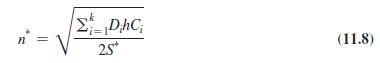
Truck capacity can also be included in this setting by comparing the total load for the opti­mal n* with truck capacity. If the optimal load exceeds truck capacity, n* is increased until the load equals truck capacity. By applying Equation 11.8 for different values of k, we can also find the optimal number of items or suppliers to be aggregated in a single delivery.

In Example 11-4, we consider the case in which the product managers at Best Buy jointly order all three models each time they place an order (see worksheet Example 11-4).

EXAMPLE 11-4 Products Ordered and Delivered Jointly

Consider the Best Buy data in Example 11-3. The three product managers have decided to aggre­gate and order all three models each time they place an order. Evaluate the optimal lot size for each model.

Analysis:

Because all three models are included in each order, the combined order cost is S* = S + s_L + s_M + s_H = $ 7,000 per order

The optimal order frequency is obtained using Equation 11.7 and is given by

Thus, if each model is to be included in every order and delivery, the product managers at Best Buy should place 9.75 orders each year. In this case, the ordering policies and costs are as shown in Table 11-2.

Because 9.75 orders are placed each year and each order costs a total of $7,000, we have

Annual order cost = 9.75 X 7,000 = $ 68,250

The annual ordering and holding cost, across the three sizes, of the aforementioned policy is given by

Annual ordering and holding cost = $ 61,512 + $ 6,151 + $ 615 + $ 68,250 = $136,528

Observe that the product managers at Best Buy lower the annual cost from $155,140 to $136,528 by ordering all products jointly. This represents a decrease of about 12 percent.

In Example 11-5, we consider optimal aggregation of orders or deliveries in the presence of capacity constraints (see worksheet Example 11-5).

EXAMPLE 11-5 Aggregation with Capacity Constraint

W.W. Grainger sources from hundreds of suppliers and is considering the aggregation of inbound shipments to lower costs. Truckload shipping costs $500 per truck along with $100 per pickup. Average annual demand from each supplier is 10,000 units. Each unit costs $50 and Grainger incurs a holding cost of 20 percent. What is the optimal order frequency and order size if Grainger decides to aggregate four suppliers per truck? What is the optimal order size and frequency if each truck has a capacity of 2,500 units?

Analysis:

In this case, W.W. Grainger has the following inputs:

Demand per product, D_t = 10,000

Holding cost, h = 0.2

Unit cost per product, Ci = $50

Common order cost, S = $500

Supplier-specific order cost, s = $100

The combined order cost from four suppliers is given by

S* = S + s₁ + s₂ + s₃ + s₄ = $ 900per order

From Equation 11.8, the optimal order frequency is

It is thus optimal for Grainger to order 14.91 times per year. The annual ordering cost per supplier is

The quantity ordered from each supplier is Q = 10,000/14.91 = 671 units per order. The annual holding cost per supplier is

This policy, however, requires a total capacity per truck of 4 X 671 = 2,684 units. Given a truck capacity of 2,500 units, the order frequency must be increased to ensure that the order quantity from each supplier is 2,500/4 = 625. Thus, W.W. Grainger should increase the order frequency to 10,000/625 = 16. The limited truck capacity results in an optimal order frequency of 16 orders per year instead of 14.91 orders per year when truck capacity was ignored. The lim­ited truck capacity will increase the annual order cost per supplier to $3,600 and decrease the annual holding cost per supplier to $3,125.

The main advantage of ordering all products jointly is that the system is easy to administer and implement. The disadvantage is that it is not selective enough in combining the particular models that should be ordered together. If product-specific order costs are high and products vary significantly in terms of their sales, it is possible to lower costs by being selective about the products
being aggregated in a joint order.

Next, we consider a policy under which the product managers do not necessarily order all models each time an order is placed, but still coordinate their orders. Lots are Ordered and Delivered Jointly for a Selected Subset of the Products We first illustrate how being selective in aggregating orders into a single order can lower costs. Consider Example 11-4, in which the manager decides to aggregate all three computer models in every order. The optimal policy from Example 11-4 is to order 9.75 times a year. The disadvantage of this policy is that the Heavypro, with annual demand of only 120 units, is also ordered 9.75 times. Given that a model-specific cost of $1,000 is incurred with each order, we are essentially adding 1,000/(120/9.75) = $81.25 in order cost to each Heavypro. If we were to include the Heavypro in every fourth order (instead of every order), though, we would save 9,750 : (3/4) = $7,312.50 in product-specific ordering cost (save three out of four product-specific orders) while incurring an additional 500 : 0.2 : [(120/9.75)/2] : 3 = $1,846.15 in holding cost (because the lot size of Heavypro would increase from 120/9.75 to [120 : (4/9.75)]. Such a policy would thus decrease the annual cost relative to complete aggregation by more than $5,466. This example points to the value of being more selective when aggregating orders.

We now discuss a procedure that is more selective in combining products to be ordered jointly. The procedure we discuss here does not necessarily provide the optimal solution. It does, however, yield an ordering policy whose cost is close to optimal. The approach of the procedure
is to first identify the “most frequently” ordered product that is included in every order. The base fixed cost S is then entirely allocated to this product. For each of the “less frequently” ordered products i, the ordering frequency is determined using only the product-specific ordering cost si. The frequencies are then adjusted so that each product i is included every mi orders, where mi is an integer. We now detail the procedure used.

We first describe the procedure in general and then apply it to the specific example. Assume that the products are indexed by i, where i varies from 1 to l (assuming a total of l products). Each product i has an annual demand Di, a unit cost Ci, and a product-specific order cost si. The common order cost is S.

Step 1: As a first step, identify the most frequently ordered product, assuming each product is ordered independently. In this case, a fixed cost of S + s, is allocated to each product. For each product i (using Equation 11.6), evaluate the ordering frequency:

This is the frequency at which product i would be ordered if it were the only product being ordered (in which case a fixed cost of S + s, would be incurred per order). Let _ be the frequency of the most frequently ordered product, i*; that is, _* is the maximum among all ni (n = ni* = max {ni, i = 1, …, l}). The most frequently ordered product is i^*, which is included each time an order is placed.

Step 2: For all products i # i*, evaluate the ordering frequency:

ni represents the desired order frequency if product i incurs the product-specific fixed cost si only each time it is ordered.

Step 3: Our goal is to include each product i # i* with the most frequently ordered product i* after an integer number of orders. For all i # i*, evaluate the frequency of product i relative to the most frequently ordered product i* to be m_i, where

In this case, [] is the operation that rounds a fraction up to the closest integer. Product i is included with the most frequently ordered product i^* every m_i orders. Given that the most frequently ordered product i* is included in every order, mi* = 1.

Step 4: Having decided the ordering frequency of each product i, recalculate the ordering frequency of the most frequently ordered product i^* to be _, where

Note that n is a better ordering frequency for the most frequently ordered product i^* than n because it takes into account the fact that each of the other products i is included with i^* every mi orders.

Step 5: For each product, evaluate an order frequency of ni = n/mi and the total cost of such an ordering policy. The total annual cost is given by

This procedure results in tailored aggregation, with higher-demand products ordered more frequently and lower-demand products ordered less frequently. Example 11-6 (see worksheet Example 11-6) considers tailored aggregation for the Best Buy ordering decision in Example 11-3.

EXAMPLE 11-6 Lot Sizes Ordered and Delivered Jointly for a Selected Subset That Varies by Order

Consider the Best Buy data in Example 11-3. Product managers have decided to order jointly, but to be selective about which models they include in each order. Evaluate the ordering policy and costs using the procedure discussed previously.

Analysis:

Recall that S = $4,000, s_L = $1,000, s_M = $1,000, s_H = $1,000. Applying Step 1, we obtain

Clearly, Litepro is the most frequently ordered model. Thus, we set n = 11.0.

We now apply Step 2 to evaluate the frequency with which Medpro and Heavypro are included with Litepro in the order. We first obtain

Next, we apply Step 3 to evaluate

Thus, Medpro is included in every second order and Heavypro is included in every fifth order (Litepro, the most frequently ordered model, is included in every order). Now that we have decided on the ordering frequency of each model, apply Step 4 (Equation 11.9) to recalculate the ordering frequency of the most frequently ordered model as

Thus, the Litepro is ordered 11.47 times per year. Next, we apply Step 5 to obtain an order­ing frequency for each product:

n_L = 11.47/year, n_M = 11.47 /2 = 5.74/ year, and n_H = 11.47 / 5 = 2.29/year

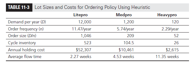
The ordering policies and resulting costs for the three products are shown in Table 11-3.

The annual holding cost of this policy is $65,383.50. The annual order cost is given by

nS + n_Ls_L + n_Ms_M + n_Hs_H = $ 65,383.50

The total annual cost is thus equal to $130,767. Tailored aggregation results in a cost reduction of $5,761 (about 4 percent) compared with the joint ordering of all models. The cost reduction results because each model-specific fixed cost of $1,000 is not incurred with every order.

From the Best Buy examples, it follows that aggregation can provide significant cost savings and reduction in cycle inventory in the supply chain. When product-specific order costs (si) are small relative to the fixed cost S, complete aggregation, whereby every product is included in every order, is very effective. Tailored aggregation provides little additional value in this setting and may not be worth the additional complexity. If Examples 11-3, 11-4, and 11-6 are repeated with s_i = $300 (change cells D5:D7 in worksheet Example 11-3 to 300), we find that tailored aggregation decreases costs by only about 1 percent relative to complete aggregation, whereas complete aggregation decreases costs by more than 25 percent relative to no aggregation. As product-specific order costs increase, however, tailored aggregation becomes more effective. If Examples 11-3, 11-4, and 11-6 are repeated with s_i = $3,000 (change cells D5:D7 in worksheet Example 11-3 to 3,000), we find that complete aggregation actually increases costs relative to no aggregation. Tailored aggregation, however, decreases costs by about 10 percent relative to no aggregation. In general, complete aggregation should be used when product-specific order costs are small, and tailored aggregation should be used when product-specific order costs are large.

Next, we consider lot sizes when material cost displays economies of scale.

Key Point

A key to reducing cycle inventory is the reduction of lot size. A key to reducing lot size without increas­ing costs is reducing the fixed cost associated with each lot. This may be achieved by reducing the fixed cost itself or by aggregating lots across multiple products, customers, or suppliers. When aggregating across multiple products, customers, or suppliers, simple aggregation is effective when product-specific order costs are small, and tailored aggregation is best if product-specific order costs are large.

Source: Chopra Sunil, Meindl Peter (2014), Supply Chain Management: Strategy, Planning, and Operation, Pearson; 6th edition.