Consumer Preferences

Given both the vast number of goods and services that our industrial economy provides for purchase and the diversity of personal tastes, how can we describe consumer preferences in a coherent way? Let’s begin by thinking about how a consumer might compare different groups of items available for purchase. Will one group of items be preferred to another group, or will the consumer be indif- ferent between the two groups?

1. Market Baskets

We use the term market basket to refer to such a group of items. Specifically, a market basket is a list with specific quantities of one or more goods. A mar- ket basket might contain the various food items in a grocery cart. It might also refer to the quantities of food, clothing, and housing that a consumer buys each month. Many economists also use the word bundle to mean the same thing as market basket.

How do consumers select market baskets? How do they decide, for example, how much food versus clothing to buy each month? Although selections may occasionally be arbitrary, as we will soon see, consumers usually select market baskets that make them as well off as possible.

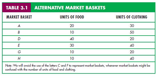
Table 3.1 shows several market baskets consisting of various amounts of food and clothing purchased on a monthly basis. The number of food items can be measured in any number of ways: by total number of containers, by number of packages of each item (e.g., milk, meat, etc.), or by number of pounds or grams. Likewise, clothing can be counted as total number of pieces, as number of pieces of each type of clothing, or as total weight or volume. Because the method of measurement is largely arbitrary, we will simply describe the items in a market basket in terms of the total number of units of each commodity. Market basket A, for example, consists of 20 units of food and 30 units of clothing, basket B consists of 10 units of food and 50 units of clothing, and so on.

To explain the theory of consumer behavior, we will ask whether consumers prefer one market basket to another. Note that the theory assumes that consumers’ preferences are consistent and make sense. We explain what we mean by these assumptions in the next subsection.

2. Some Basic Assumptions about Preferences

The theory of consumer behavior begins with three basic assumptions about people’s preferences for one market basket versus another. We believe that these assumptions hold for most people in most situations.

1. Completeness: Preferences are assumed to be complete. In other words, consumers can compare and rank all possible baskets. Thus, for any two market baskets A and B, a consumer will prefer A to B, will prefer B to A, or will be indifferent between the two. By indifferent we mean that a per- son will be equally satisfied with either basket. Note that these preferences ignore costs. A consumer might prefer steak to hamburger but buy ham- burger because it is cheaper.
2. Transitivity: Preferences are transitive. Transitivity means that if a consumer prefers basket A to basket B and basket B to basket C, then the consumer also prefers A to C. For example, if a Porsche is preferred to a Cadillac and a Cadillac to a Chevrolet, then a Porsche is also preferred to a Chevrolet. Transitivity is normally regarded as necessary for consumer consistency.
3. More is better than less: Goods are assumed to be desirable—i.e., to be good. Consequently, consumers always prefer more of any good to less. In addi- tion, consumers are never satisfied or satiated; more is always better, even if just a little better.1 This assumption is made for pedagogic reasons; name- ly, it simplifies the graphical analysis. Of course, some goods, such as air pollution, may be undesirable, and consumers will always prefer less. We ignore these “bads” in the context of our immediate discussion of consumer choice because most consumers would not choose to purchase them. We will, however, discuss them later in the chapter.

These three assumptions form the basis of consumer theory. They do not explain consumer preferences, but they do impose a degree of rationality and reasonableness on them. Building on these assumptions, we will now explore consumer behavior in greater detail.

3. Indifference Curves

We can show a consumer ’s preferences graphically with the use of indifference curves. An indifference curve represents all combinations of market baskets that pro- vide a consumer with the same level of satisfaction. That person is therefore indiffer- ent among the market baskets represented by the points graphed on the curve.

Given our three assumptions about preferences, we know that a consumer can always indicate either a preference for one market basket over another or indifference between the two. We can then use this information to rank all pos- sible consumption choices. In order to appreciate this principle in graphic form, let’s assume that there are only two goods available for consumption: food F and clothing C. In this case, all market baskets describe combinations of food and clothing that a person might wish to consume. As we have already seen, Table 3.1 provides some examples of baskets containing various amounts of food and clothing.

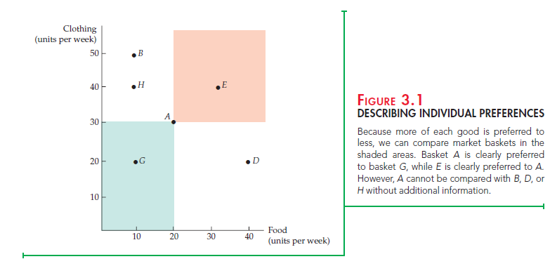
In order to graph a consumer ’s indifference curve, it helps first to graph his or her individual preferences. Figure 3.1 shows the same baskets listed in Table 3.1. The horizontal axis measures the number of units of food purchased each week; the vertical axis measures the number of units of clothing. Market basket A, with

20 units of food and 30 units of clothing, is preferred to basket G because A con- tains more food and more clothing (recall our third assumption that more is better than less). Similarly, market basket E, which contains even more food and even more clothing, is preferred to A. In fact, we can easily compare all market baskets in the two shaded areas (such as E and G) to A because they contain either more or less of both food and clothing. Note, however, that B contains more cloth- ing but less food than A. Similarly, D contains more food but less clothing than A. Therefore, comparisons of market basket A with baskets B, D, and H are not possible without more information about the consumer ’s ranking.

This additional information is provided in Figure 3.2, which shows an indiffer- ence curve, labeled U1, that passes through points A, B, and D. This curve indi- cates that the consumer is indifferent among these three market baskets. It tells us that in moving from market basket A to market basket B, the consumer feels neither better nor worse off in giving up 10 units of food to obtain 20 additional units of clothing. Likewise, the consumer is indifferent between points A and D: He or she will give up 10 units of clothing to obtain 20 more units of food. On the other hand, the consumer prefers A to H, which lies below U1.

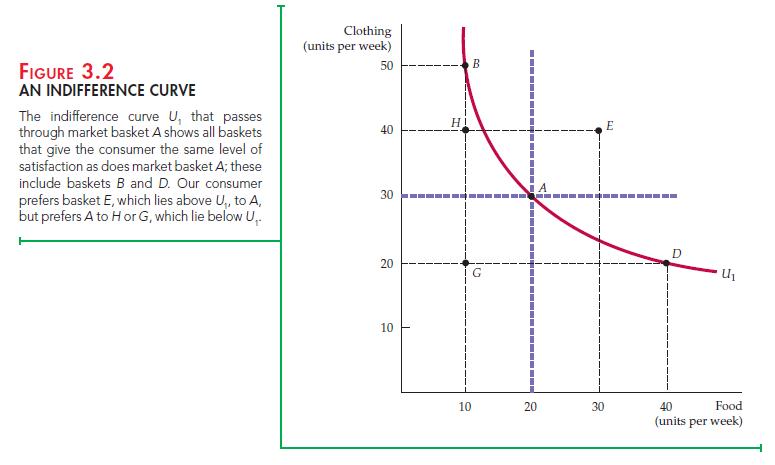
Note that the indifference curve in Figure 3.2 slopes downward from left to right. To understand why this must be the case, suppose instead that it sloped upward from A to E. This would violate the assumption that more of any commodity is preferred to less. Because market basket E has more of both food and clothing than market basket A, it must be preferred to A and therefore cannot be on the sameindifference curve as A. In fa ct, any market basket lying above and to the right of indifference curve U1 in Figure 3.2 is preferred to any market basket on U1.

4. Indifference Maps

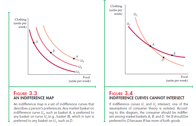
To describe a person’s preferences for all combinations of food and clothing, we can graph a set of indifference curves called an indifference map. Each indif- ference curve in the map shows the market baskets among which the person is indifferent. Figure 3.3 shows three indifference curves that form part of an indifference map (the entire map includes an infinite number of such curves). Indifference curve U3  generates the highest level of satisfaction, followed by indifference curves U2 and U1.

Indifference curves cannot intersect. To see why, we will assume the con- trary and see how the resulting graph violates our assumptions about consumer behavior. Figure 3.4 shows two indifference curves, U1  and U2, that intersect at A. Because A and B are both on indifference curve U1, the consumer must be indifferent between these two market baskets. Because both A and D lie on indifference curve U2, the consumer is also indifferent between these market baskets. Consequently, using the assumption of transitivity, the consumer is also indifferent between B and D. But this conclusion can’t be true: Market basket B must be preferred to D because it contains more of both food and clothing. Thus, intersecting indifference curves contradicts our assumption that more is preferred to less.

Of course, there are an infinite number of nonintersecting indifference curves, one for every possible level of satisfaction. In fact, every possible market basket (each corresponding to a point on the graph) has an indifference curve passing through it.

5. The Shape of Indifference Curves

Recall that indifference curves are all downward sloping. In our example of food and clothing, when the amount of food increases along an indifference curve, the amount of clothing decreases. The fact that indifference curves slope downward follows directly from our assumption that more of a good is better than less. If an indifference curve sloped upward, a consumer would be indif- ferent between two market baskets even though one of them had more of both food and clothing.

As we saw in Chapter 1, people face trade-offs. The shape of an indifference curve describes how a consumer is willing to substitute one good for another. Look, for example, at the indifference curve in Figure 3.5. Starting at market basket A and moving to basket B, we see that the consumer is willing to give up 6 units of clothing to obtain 1 extra unit of food. However, in moving from B to D, he is willing to give up only 4 units of clothing to obtain an additional unit of food; in moving from D to E, he will give up only 2 units of clothing for 1 unit of food. The more clothing and the less food a person consumes, the more cloth- ing he will give up in order to obtain more food. Similarly, the more food that a person possesses, the less clothing he will give up for more food.

6. The Marginal Rate of Substitution

To quantify the amount of one good that a consumer will give up to obtain more of another, we use a measure called the marginal rate of substitution (MRS). The MRS of food F for clothing C is the maximum amount of clothing that a person is willing to give up to obtain one additional unit of food. Suppose, for example, the MRS is 3. This means that the consumer will give up 3 units of clothing to obtain 1 additional unit of food. If the MRS is 1/2,  the consumer is willing to give up only 1/2  unit of clothing. Thus, the MRS measures the value that the individual places on 1 extra unit of a good in terms of another.

Look again at Figure 3.5. Note that clothing appears on the vertical axis and food on the horizontal axis. When we describe the MRS, we must be clear about which good we are giving up and which we are getting more of. To be consistent throughout the book, we will define the MRS in terms of the amount of the good on the vertical axis that the consumer is willing to give up in order to obtain 1 extra unit of the good on the horizontal axis. Thus, in Figure 3.5 the MRS refers to the amount of clothing that the consumer is willing to give up to obtain an additional unit of food. If we denote the change in clothing by 6.C and the change in food by 6.F, the MRS can be written as – 6. C/6.F. We add the negative sign to make the marginal rate of substitution a positive num- ber. (Remember that 6.C is always negative; the consumer gives up clothing to obtain additional food.)

Thus the MRS at any point is equal in magnitude to the slope of the indiffer- ence curve. In Figure 3.5, for example, the MRS between points A and B is 6: The consumer is willing to give up 6 units of clothing to obtain 1 additional unit of food. Between points B and D, however, the MRS is 4: With these quantities of food and clothing, the consumer is willing to give up only 4 units of clothing to obtain 1 additional unit of food.

CONVEXITY Also observe in Figure 3.5 that the MRS falls as we move down the indifference curve. This is not a coincidence. This decline in the MRS reflects an important characteristic of consumer preferences. To understand this, we will add an additional assumption regarding consumer preferences to the three that we discussed earlier in this chapter (see page 70):

4. Diminishing marginal rate of substitution: Indifference curves are usu- ally convex, or bowed inward. The term convex means that the slope of the indifference curve increases (i.e., becomes less negative) as we move down along the curve. In other words, an indifference curve is convex if the MRS diminishes along the curve. The indifference curve in Figure 3.5 is convex. As we have seen, starting with market basket A in Figure 3.5 and moving to basket B, the MRS of food F for clothing C is – 6.C/6.F = – ( – 6)/1  = 6. However, when we start at basket B and move from B to D, the MRS falls to 4. If we start at basket D and move to E, the MRS is 2. Starting at E and moving to G, we get an MRS of 1. As food consumption increases, the slope of the indifference curve falls in magnitude. Thus the MRS also falls.2

Is it reasonable to expect indifference curves to be convex? Yes. As more and more of one good is consumed, we can expect that a consumer will prefer to give up fewer and fewer units of a second good to get additional units of the first one. As we move down the indifference curve in Figure 3.5 and consump- tion of food increases, the additional satisfaction that a consumer gets from still more food will diminish. Thus, he will give up less and less clothing to obtain additional food.

Another way of describing this principle is to say that consumers generally prefer balanced market baskets to market baskets that contain all of one good and none of another. Note from Figure 3.5 that a relatively balanced market bas- ket containing 3 units of food and 6 units of clothing (basket D) generates as much satisfaction as another market basket containing 1 unit of food and 16 units of clothing (basket A). It follows that a balanced market basket containing, for example, 6 units of food and 8 units of clothing will generate a higher level of satisfaction.

7. Perfect Substitutes and Perfect Complements

The shape of an indifference curve describes the willingness of a consumer to substitute one good for another. An indifference curve with a different shape implies a different willingness to substitute. To see this principle, look at the two somewhat extreme cases illustrated in Figure 3.6.

In §2.1, we explain that two goods are substitutes when an increase in the price of one leads to an increase in the quantity demanded of the other. 2With nonconvex preferences, the MRS increases as the amount of the good measured on the hori- zontal axis increases along any indifference curve. This unlikely possibility might arise if one or both goods are addictive. For example, the willingness to substitute an addictive drug for other goods might increase as the use of the addictive drug increased.

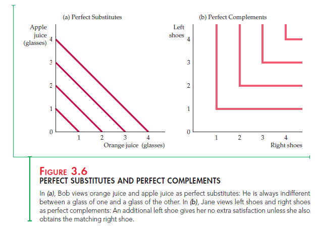
Figure 3.6 (a) shows Bob’s preferences for apple juice and orange juice. These two goods are perfect substitutes for Bob because he is entirely indiffer- ent between having a glass of one or the other. In this case, the MRS of apple juice for orange juice is 1: Bob is always willing to trade 1 glass of one for 1 glass of the other. In general, we say that two goods are perfect substitutes when the marginal rate of substitution of one for the other is a constant. Indifference curves describing the trade-off between the consumption of the goods are straight lines. The slope of the indifference curves need not be -1 in the case of perfect substitutes. Suppose, for example, that Dan believes that one 16-megabyte memory chip is equivalent to two 8-megabyte chips because both combinations have the same memory capacity. In that case, the slope of Dan’s indifference curve will be -2 (with the number of 8-megabyte chips on the vertical axis).

Figure 3.6 (b) illustrates Jane’s preferences for left shoes and right shoes. For Jane, the two goods are perfect complements because a left shoe will not increase her satisfaction unless she can obtain the matching right shoe. In this case, the MRS of left shoes for right shoes is zero whenever there are more right shoes than left shoes; Jane will not give up any left shoes to get additional right shoes. Correspondingly, the MRS is infinite whenever there are more left shoes than right because Jane will give up all but one of her excess left shoes in order to obtain an additional right shoe. Two goods are perfect complements when the indifference curves for both are shaped as right angles.

BADS So far, all of our examples have involved products that are “goods”—i.e., cases in which more of a product is preferred to less. However, some things are bads: Less of them is preferred to more. Air pollution is a bad; asbestos in housing insulation is another. How do we account for bads in the analysis of consumer preferences?

The answer is simple: We redefine the product under study so that consumer tastes are represented as a preference for less of the bad. This reversal turns the bad into a good. Thus, for example, instead of a preference for air pollution, we will discuss the preference for clean air, which we can measure as the degree of reduction in air pollution. Likewise, instead of referring to asbestos as a bad, we will refer to the corresponding good, the removal of asbestos.

With this simple adaptation, all four of the basic assumptions of consumer theory continue to hold, and we are ready to move on to an analysis of consumer budget constraints.

Source: Pindyck Robert, Rubinfeld Daniel (2012), Microeconomics, Pearson, 8th edition.