Main Effects in Experimental Research

For observation of the main effects, we import the data in Table 9.1, augmented with some derived, additional information, now shown in Table 9.2.

We observed in Figure 9.1 that there is practically no interac­tion between the factors a and b, but that has no bearing what­ever on the presence or absence of the main effects of either a or of b. Focusing on the first column of numbers in this table, we notice that a is tested for its effect four times, each time with a different level of b. The column average 8.0 is thus the average of the effect of a, tested for four times, each time associated with b. Testing the main effects of factors at three or more levels is not as simple as it is for factors at two levels. For instance, the main effect of a has three components: the effect of causing it to jump

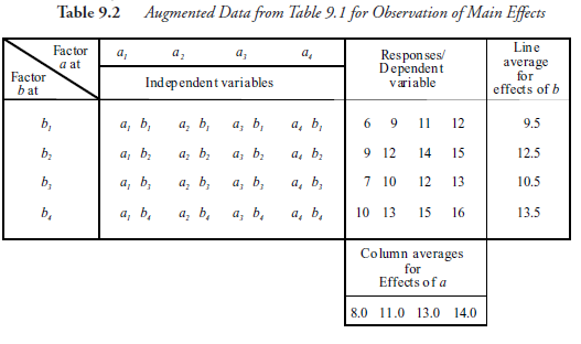
1. from level 1 to level 2
2. from level 2 to level 3
3. from level 3 to level 4

These, taken from the table, are respectively

11.0 – 8.0 = 3.0

13.0 – 11.0 = 2.0

14.0 – 13.0 = 0

Similarly, the three components of the main effect of b are

12.5 – 9.5 = 0

10.5 – 12.5 = -0

13.5 – 10.5 = 3.0

We also note that these effects are cumulative in nature. For instance, the main effect of causing b to jump from level 1 to level 3 is (12.5 — 9.5) + (10.5 — 12.5) = 1.0, which is the same as (10.5 – 9.5) = 1.0.

Though these numbers give some idea of the combined effects of multiple factors, the values of main effects, per the defi­nition, require further elaboration. Considering their impor­tance, we will take a close-up look at the main effects, using another, even more simplified example. Firstly, we note that the main effect of a factor a at level l, designated d]_, acting in combi­nation with other factors, by definition, is the difference between the mean of all the values of the dependent variable at aj and the grand mean of all the values of the dependent variable in the entire factorial experiment. Using only two independent vari­ables, a and b, both quantitative, acting at only three levels, the main effects, using fictitious numbers, are demonstrated in Table 9.3. Symbols a and @ are used for the main effects of factors a and b, respectively; subscripts with a and @, as with the indepen­dent variables, indicate the levels.

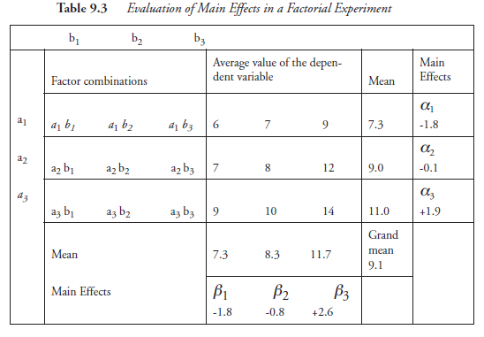
Denoting Table 9.3 as a (3 x 3) factorial, we may think of other factorials, such as (3 x 2), (2 x 3), (3 x 4), (4 x 2), and so on. The same method as that used in the table of evaluating the main effects for these holds good. Each of the values in the table, indicated as main effects, corresponds to the factor at one level. For practical purposes, though, the so-called differential main effects are more significant; those show the difference in values of the main effects at two different levels of a given factor. Three typical examples are tabulated below.

Differential main

effect of factor . . . between levels . . .                                is

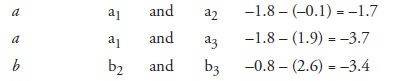
The values of the main effects and the differential main effects being negative need not concern us because the improvement in the dependent variable may be either an increase or decrease in its value based on what it represents.

Source: Srinagesh K (2005), The Principles of Experimental Research, Butterworth-Heinemann; 1st edition.