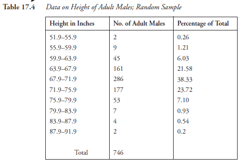
Let us say that statistics were required on the height of adult males in the United States. The usual, established, statistical procedures take over. Because, obviously, it is not practical to reach every adult male in the country, an appropriate random sampling is adapted. The hypothetical data obtained and tabulated in Table 17.4 is where we start.
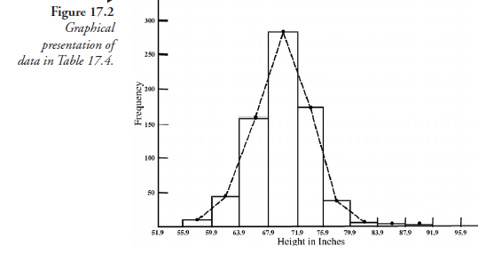
This same data is shown graphically in Figure 17.2, which, as we recall, is a typical frequency histogram. The lines joining the class marks in this figure show the tendency toward normal distribution. If the classes were taken with narrow widths (class ranges), for instance, an increment of 1 inch instead of 4 inches, the tendency toward normal distribution would be even more obvious. We will assume at this point, which is reasonable, that with more individuals in the sample than the present 746 and with narrower increments in height (on the abscissa) in the figure, the data will approximate to normal distribution.
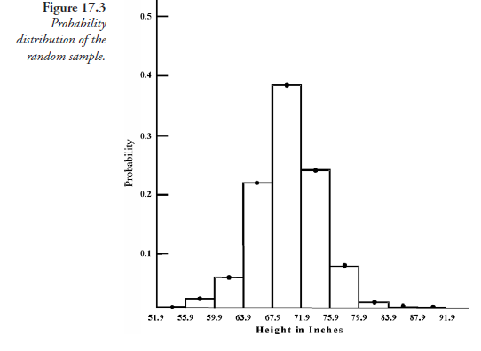
Thus far, we note, our consideration is confined to statistics, as if it were free of probability. We now recall that in the process of random sampling, the element of chance was operative without hindrance. That there should be a given number in each class, for instance, 161 individuals with height between 63.9 and 67.9 inches, was a matter of pure chance. Stated differently, the probability of finding 161 adult males in the population with the height between 63.9 and 67.9 inches, judging from the present sample, was 161 ÷ 746. On this basis, we can now assign probability values for each class and prepare Figure 17.3 and justifiably call it a probability distribution for the random sample.
The same data are shown graphically in Figure 17.4. The abscissas in this figure, as in Figure 17.2, are classes of height, but the ordinates are not the frequency distribution; instead, they are measures of the probability of finding adult males with the corresponding ranges in heights. Each ordinate in this graphical relation may be considered as the probability function of the corresponding class width; for instance, the probability function of height 71.9 to 75.9 inches is 177 ÷ 746. This probability can be expressed, using p (instead of the conventional f) in the functional relation:
p (71.9-75.9 in) = 177÷746
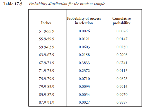
Further, we note that the values of probability functions, given by the height of bars, vary along the classes of the random variable (on the abscissa). This fact may be expressed as the probability having different densities as we proceed from one end of the variable to the other. Starting at the lowest density of 0.0026 for the variable at 51.9 to 55.9 inches, the density increases to a maximum of 0.3833 at 67.9 to 71.9 inches, then decreases to the lowest value of 0.0027 at 87.9 to 91.9 inches. Conforming to this observation, Figure 17.4 is more appropriately referred to as a probability density distribution.
For the data in Figure 17.3, we can also plot a cumulative distribution of probability curve as shown in Figure 17.4.
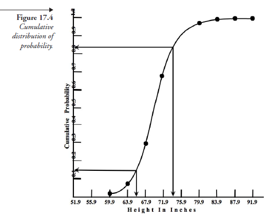
This curve is suitable for answering such questions as
- What is the probability that the height of all adult males in the United States is above 75.9 inches? The answer to this question is 1 – 0.9 = 1 (or 10 percent).
- What is the probability that such height is below 59.9 inches? It is 0.025 (or 2.5 percent).
Note that the sum of all the probabilities (of success) in Table 17.5, which is also the probability corresponding to the maximum height in Figure 17.4, is 1.0. As we pointed out earlier, relative to normal distribution, the number of “bars” in the histogram (Figure 17.3) can be increased by decreasing the class widths (on the abscissa), thereby making the lines joining the probability values tend to be smooth, approximating the shape of normal distribution. Then, the sum of the areas of all the bars, together, which in the limit is the curve, is 1.0. In summary, we may say that the area under the curve of the probability density distribution, or the probability functions of a given random variable in a sample (or in a population), is unity. We also note that the data for the frequency distribution (Figure 17.2) and that of the probability density (Figure 17.4), if both are approximated to normal distribution, present similar curves. The only difference is in the scale of the ordinates. Whereas the ordinates for frequency distribution are in discrete numbers of elements within different classes, for probability density, the ordinates are in fractions or percentages, if we prefer, showing the probabilities of success of different classes.
Source: Srinagesh K (2005), The Principles of Experimental Research, Butterworth-Heinemann; 1st edition.
Just wish to say your article is as amazing. The clearness in your post is
simply cool and i can assume you’re an expert on this subject.
Fine with your permission let me to grab your feed to keep up to date with forthcoming post.
Thanks a million and please keep up the enjoyable
work.
I love what you guys tend to be up too. This kind of clever work and coverage!
Keep up the amazing works guys I’ve added you guys to my personal blogroll.
Great post. I will be going through a few of these issues as well..
I was able to find good advice from your blog articles.