Sequential Experimenting

As the reader should have noticed, the two key steps in designing the experiment in all the variations so far presented are (1) find­ing the number of items in the sample N, and (2) computing the criterion value, X, to compare it with the mean of the response output, X1. If the sample items are such things as specimens for hardness measurement or a group of players kicking a soccer ball, having all the N sample items together, in terms of either money or time, is not a problem. Instead, suppose the sample items to be tested are rockets of a novel design. It is prohibitively expensive both in terms of money and time to collect all N items, each with different levels of variable factors, and to fire them simulta­neously, possibly at the end of a long waiting period. Assembling each item may take a few weeks, if not longer. In such cases, experimenting with one item at a time, followed by a long prepa­ration time before the second experiment is to be done, is reason­able. Also, at the end of each test, the data is subjected to the test of significance somewhat on the same basis as, but with different details from, that of the experiment. As soon as the data passes the test of significance, the project of experimentation is termi­nated. Most often, it happens that the number of sequential tests necessary is much smaller than the number N, evaluated by com­putation. The first three steps of the procedure shown below are the same as in the previous designs, but the subsequent steps are specially formulated (by statisticians) for the situation. An exam­ple is illustrated using typical hypothetical numbers.

Example 6:

This experiment was for a metallurgical enterprise. A steel part was shipped out to a possible customer, who proposed to buy this component if it was approved as a vendor item. The parts were hardened by carbon diffusion. This process, with the present setup, required about fifteen hours of soaking in the furnace; 26 percent of the parts were rejected by the possible customer because they failed to show the required hardness of 88 HRC (Rockwell Hardness on C Scale). The measurement of hardness by the enterprise before shipping was recorded as 90 HRC with a standard deviation of four. The in-house metallurgist proposed to make certain changes in the process so that the parts could meet the customer’s requirement. The effect of one set of changes in the process could be tested for on consecutive days.

The sequential experiment begins at this point. As was shown earlier in this chapter, the procedural steps differ for the situation sets:

1. σ is known; μ0 > μ1.
2. σ is known; μ0 ≠ μ1.
3. σ is not known; μ0 > μ1.

Procedure:

The present experiment conforms to set a.

1. σ is known to be four.
2. State the hypotheses:

H0: μ1 = μ0 = 88
Hα: μ1 > μ0; this is one sided.

3. Choose α = 0.05, β = 0.025, δ = 4.
4. Find in Table 18.2, Uα = 1.645, Ub = 1.960

5. Calculate

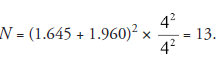
Up to this point, the procedural steps are the same as for Situ­ation Set 1. Steps from now on are different for sequential exper­iments. The numbers here onwards assigned to steps do not correspond to the same functions as in Examples 1-5.

Compute

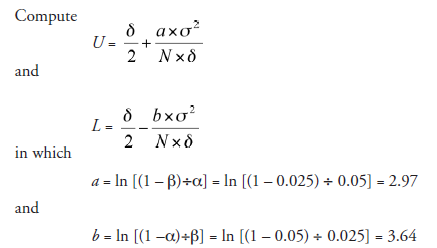
U and L for the present situation set simplify to

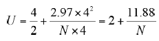
and

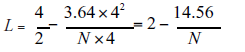
6. With formulas for U (standing for the upper) and L (standing for the lower) known, plot two lines on the same graph, corresponding to N = 1, 2, 3, 4 . . . as shown in Figure 18.2.

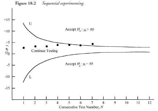
Note: These lines serve the same purpose as the criterion number, X, in Situation Set 1. After plotting these lines, one can notice that the graph area is divided into three fields. Mark these areas as shown in Figure 18.2: (1) accept Hα, (2) continue testing, and (3) Accept Hq The rest of the proce­dure is nearly the same as in Situation Set 1, except that in place of criterion number, now we have criterion lines.

7. Conduct the first experiment (N = 1), and get the output value, χ1. This is the first experiment; now X = χ1.
8. Find (X – μ0).
9. Plot this value as ordinate in the graph corre­sponding to abscissa N = 1.

Note: The location of this point, meaning the particular field of the graph in which it falls, directs the decision. If it falls in either area “accept Hα” or “accept H0,” that is the end of the experimentation. If it falls in neither, it will be in the area “continue testing.”

Then,

10. Prepare the second specimen and perform the sec­ond experiment. Let us say the output of this experiment is X2- Then,

X = (χ1 + χ2) ÷ 2
Find (X – μ0).

Plot this value in the graph corresponding to N = 2.

Again, depending on the location of this point, make a deci­sion.

Continue, if need be, with N = 3, N = 4, and so on.

The very first time a plotted point derived as above falls out­side the area “continue experiments,” the decision is accepted as final, and the project of experimentation is terminated. If the point is located in “accept Hα,” that is what the decision is; if it is “accept H0,” likewise, that is the decision.

The results of these steps, one for each N = 1, 2, 3 . . . are shown in Figure 18.2. We find that the point corresponding to the seventh test falls for the first time in the field “accept Hα.” That is the end of the experiment. Whatever changes were made in the parameters at that step will then be followed as routine in heat-treating the parts. The required number of parts processed according to the new parameters will be sent to the customer, now with new hope for approval.

Source: Srinagesh K (2005), The Principles of Experimental Research, Butterworth-Heinemann; 1st edition.