Over a Century of Capital Market History in One Easy Lesson

Financial analysts are blessed with an enormous quantity of data. There are comprehensive databases of the prices of U.S. stocks, bonds, options, and commodities, as well as huge amounts of data for securities in other countries. We focus on a study by Dimson, Marsh, and Staunton that measures the historical performance of three portfolios of U.S. securities:^[1]

1. A portfolio of Treasury bills, that is, U.S. government debt securities maturing in less than one year.^[2]
2. A portfolio of U.S. government bonds.
3. A portfolio of U.S. common stocks.

These investments offer different degrees of risk. Treasury bills are about as safe an invest­ment as you can make. There is no risk of default, and their short maturity means that the prices of Treasury bills are relatively stable. In fact, an investor who wishes to lend money for, say, three months can achieve a perfectly certain payoff by purchasing a Treasury bill matur­ing in three months. However, the investor cannot lock in a real rate of return: There is still some uncertainty about inflation.

By switching to long-term government bonds, the investor acquires an asset whose price fluctuates as interest rates vary. (Bond prices fall when interest rates rise and rise when inter­est rates fall.) An investor who shifts from bonds to common stocks shares in all the ups and downs of the issuing companies.

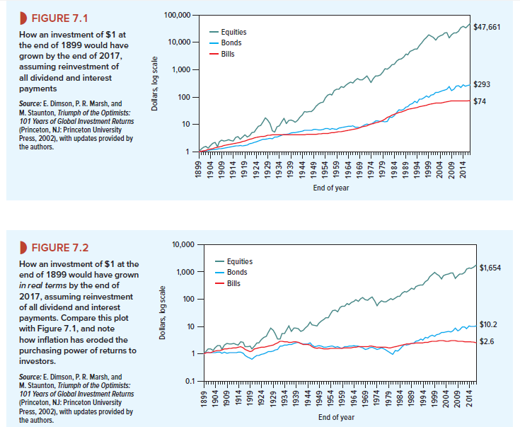
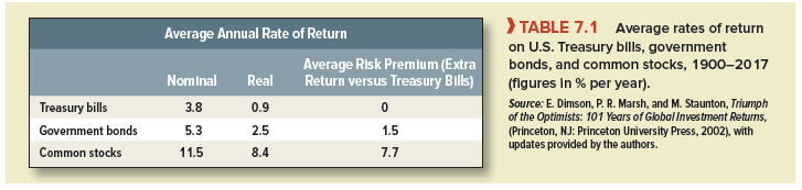
Figure 7.1 shows how your money would have grown if you had invested $1 at the end of 1899 and reinvested all dividend or interest income in each of the three portfolios.³ Figure 7.2 is identical except that it depicts the growth in the real value of the portfolio. We focus here on nominal values.

Investment performance coincides with our intuitive risk ranking. A dollar invested in the safest investment, Treasury bills, would have grown to $74 by the end of 2017, barely enough to keep up with inflation. An investment in long-term Treasury bonds would have produced $293. Common stocks were in a class by themselves. An investor who placed a dollar in the stocks of large U.S. firms would have received $47,661.

We can also calculate the rate of return from these portfolios for each year from 1900 to 2017. This rate of return reflects both cash receipts—dividends or interest—and the capital gains or losses realized during the year. Averages of the 118 annual rates of return for each portfolio are shown in Table 7.1.

Over this period, Treasury bills have provided the lowest average return—3.8% per year in nominal terms and 0.9% in real terms. In other words, the average rate of inflation over this period was about 3% per year. Common stocks were again the winners. Stocks of major corporations provided an average nominal return of 11.5%. By taking on the risk of common stocks, investors earned a risk premium of 11.5 – 3.8 = 7.7% over the return on Treasury bills.

You may ask why we look back over such a long period to measure average rates of return. The reason is that annual rates of return for common stocks fluctuate so much that averages taken over short periods are meaningless. Our only hope of gaining insights from historical rates of return is to look at a very long period.^[3]

1. Arithmetic Averages and Compound Annual Returns

Notice that the average returns shown in Table 7.1 are arithmetic averages. In other words, we simply added the 118 annual returns and divided by 118. The arithmetic average is higher than the compound annual return over the period. The 118-year compound annual return for common stocks was 9.6%.^[4]

The proper uses of arithmetic and compound rates of return from past investments are often misunderstood. Therefore, we call a brief time-out for a clarifying example.

Suppose that the price of Big Oil’s common stock is $100. There is an equal chance that at the end of the year the stock will be worth $90, $110, or $130. Therefore, the return could be -10%, +10%, or +30% (we assume that Big Oil does not pay a dividend). The expected return is / (-10 + 10 + 30) = +10%.

If we run the process in reverse and discount the expected cash flow by the expected rate of return, we obtain the value of Big Oil’s stock:

The expected return of 10% is therefore the correct rate at which to discount the expected cash flow from Big Oil’s stock. It is also the opportunity cost of capital for investments that have the same degree of risk as Big Oil.

Now suppose that we observe the returns on Big Oil stock over a large number of years. If the odds are unchanged, the return will be -10% in a third of the years, +10% in a further third, and +30% in the remaining years. The arithmetic average of these yearly returns is

Thus, the arithmetic average of the returns correctly measures the opportunity cost of capital for investments of similar risk to Big Oil stock.^[5]

The average compound annual return^[6] on Big Oil stock would be

(.9 x 1.1 x 1.3)^1/3 – 1 = .088, or 8.8%

which is less than the opportunity cost of capital. Investors would not be willing to invest in a project that offered an 8.8% expected return if they could get an expected return of 10% in the capital markets. The net present value of such a project would be

Moral: If the cost of capital is estimated from historical returns or risk premiums, use arithmetic averages, not compound annual rates of return.^[7]

2. Using Historical Evidence to Evaluate Today’s Cost of Capital

Suppose there is an investment project that you know—don’t ask how—has the same risk as Standard and Poor’s Composite Index. We will say that it has the same degree of risk as the market portfolio, although this is speaking somewhat loosely, because the index does not include all risky investments. What rate should you use to discount this project’s forecasted cash flows?

Clearly you should use the currently expected rate of return on the market portfolio; that is, the return investors would forgo by investing in the proposed project. Let us call this market return r_m. One way to estimate r_m is to assume that the future will be like the past and that today’s investors expect to receive the same “normal” rates of return revealed by the averages shown in Table 7.1. In this case, you would set r_m at 11.5%, the average of past market returns.

Unfortunately, this is not the way to do it; r_m is not likely to be stable over time. Remember that it is the sum of the risk-free interest rate rf and a premium for risk. We know that rf varies. For exam­ple, in 1981 the interest rate on Treasury bills was about 15%. It is difficult to believe that investors in that year were content to hold common stocks offering an expected return of only 11.5%.

If you need to estimate the return that investors expect to receive, a more sensible procedure is to take the interest rate on Treasury bills and add 7.7%, the average risk premium shown in Table 7.1. For example, suppose that the current interest rate on Treasury bills is 2%. Adding on the average risk premium gives

r_m = r_f + normal risk premium = .02 + .077 = .097, or 9.7%

The crucial assumption here is that there is a normal, stable risk premium on the market portfolio, so that the expected future risk premium can be measured by the average past risk premium.

Even with more than 100 years of data, we can’t estimate the market risk premium exactly; nor can we be sure that investors today are demanding the same reward for risk that they were 50 or 100 years ago. All this leaves plenty of room for argument about what the risk premium really is.^[8]

Many financial managers and economists believe that long-run historical returns are the best measure available. Others have a gut instinct that investors don’t need such a large risk premium to persuade them to hold common stocks.^[9] For example, surveys of businesspeople and academics commonly suggest that they expect a market risk premium that is somewhat below the historical average.^[10]

If you believe that the expected market risk premium is less than the historical average, you probably also believe that history has been unexpectedly kind to investors in the United States and that this good luck is unlikely to be repeated. Here are two reasons that history may overstate the risk premium that investors demand today.

Reason 1 Since 1900, the United States has been among the world’s most prosperous coun­tries. Other economies have languished or been wracked by war or civil unrest. By focusing on equity returns in the United States, we may obtain a biased view of what investors expected. Perhaps the historical averages miss the possibility that the United States could have turned out to be one of those less-fortunate countries.^[11]

Figure 7.3 sheds some light on this issue. It is taken from a comprehensive study by Dimson, Marsh, and Staunton of market returns in 20 countries and shows the average risk premium in each country between 1900 and 2017. There is no evidence here that U.S. inves­tors have been particularly fortunate; the United States was just about average in terms of the risk premium.

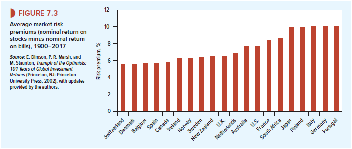
In Figure 7.3, Swiss stocks come bottom of the league; the average risk premium in Switzerland was only 5.5%. The clear winner was Portugal, with a premium of 10.0%. Some of these differences between countries may reflect differences in risk. But remember how difficult it is to make precise estimates of what investors expected. You probably would not be too far out if you concluded that the expected risk premium was the same in each country.^[12]

Reason 2 Economists who believe that history may overstate the return that investors expect often point to the fact that stock prices in the United States have for some years outpaced the growth in company dividends or earnings.

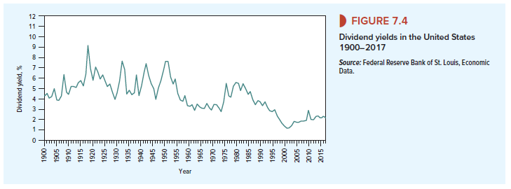
Figure 7.4 plots dividend yields in the United States from 1900 to 2017. At the start of the period, the yield was 4.4%. By 1917, it had risen to just over 10.0%, but from then onward, there was a clear, long-term decline. By 2017, yields had fallen to 1.9%. It seems unlikely that investors expected this decline in yields, in which case, some part of the actual return during this period was unexpected.^[13]

How should we interpret the decline in yields? Suppose that investors expect a steady growth (g) in a stock’s dividend. Then its value is PV = DIVy(r – g), and its dividend yield is DIV^PV = r – g. In this case, the dividend yield measures the difference between the discount rate and the expected growth rate. So, if we observe that dividend yields decline, it could either be because investors have increased their forecast of future growth or because they are content with a lower expected return.

What’s the answer? Have investors raised their forecast of future dividend growth? One possibility is that they now anticipate a forthcoming golden age of prosperity and surging profits. But a simpler (and more plausible) argument is that companies have increasingly preferred to distribute cash by stock repurchase. As we explain in Chapter 16, the effect of using cash to buy back stock is to reduce the current dividend yield and to increase the future rate of dividend growth. The dividend yield is lower but the expected return is unchanged.

What about the second possibility? Could a decline in risk have caused investors to be satisfied with a lower rate of return? A few years ago, you would likely hear people say that improvements in economic management have made investment in the stock market less risky than it used to be. Since the financial crisis of 2007-2009, investors are less sure that this is the case. But perhaps the growth in mutual funds has made it easier for individuals to diver­sify away part of their risk, or perhaps pension funds and other financial institutions have found that they also could reduce their risk by investing part of their funds overseas. If these investors can eliminate more of their risk than in the past, they may be content with a lower risk premium.

The effect of any decline in the expected market risk premium is to increase the realized rate of return. Suppose that the stocks in the Standard & Poor’s Index pay an aggregate dividend of $400 billion (DIV₁ = 400) and that this dividend is expected to grow indefinitely at 6% per year (g = .06). If the yield on these stocks is 2%, the expected total rate of return is r = 6 + 2 = 8%. If we plug these numbers into the constant-growth dividend-discount model, then the value of the market portfolio is PV = DIV₁/(r – g) = 400/(.08 – .06) = $20,000 billion, approximately its actual total value in 2017.

The required return of 8%, of course, includes a risk premium. For example, if the risk-free interest rate is 1%, the risk premium is 7%. Suppose that investors now see the stock market as a safer investment than before. Therefore, they revise their required risk premium downward from 7% to 6.5% and the required return from 8% to 7.5%. As a result the value of the market portfolio increases to PV = DIV₁/(r – g) = 400/(.075 – .06) = $26,667 billion, and the dividend yield falls to DIV₁/PV = 400/26,667 = .015 or 1.5%.

Thus a fall of 0.5 percentage point in the risk premium that investors demand would cause a 33% rise in market value, from $20,000 to $26,667 billion. The total return to investors when this happens, including the 2% dividend yield, is 2 + 33 = 35%. With a 1% interest rate, the risk premium earned is 35 – 1 = 34%, much greater than investors expected. If and when this 34% risk premium enters our sample of past risk premiums, we may be led to a double mistake. First, we will overestimate the risk premium that investors required in the past. Second, we will fail to recognize that investors require a lower expected risk premium when they look to the future.

Out of this debate only one firm conclusion emerges: Trying to pin down an exact number for the market risk premium is about as hopeless as eating spaghetti with a one-pronged fork.

History contains some clues, but ultimately, we have to judge whether investors on average have received what they expected. Many financial economists rely on the evidence of history and therefore work with a risk premium of about 7%. The remainder generally use a some­what lower figure. Brealey, Myers, and Allen have no official position on the issue, but we believe that a range of 5% to 8% is reasonable for the risk premium in the United States.

Source:  Brealey Richard A., Myers Stewart C., Allen Franklin (2020), Principles of Corporate Finance, McGraw-Hill Education; 13th edition.