Procedural Steps in Structural Equation Modelling

Structural equation modelling includes six key steps. In addition to data collection, the steps are model specification, identification, estimation, evaluation and modification (Fig. 3.1).

1. Model Specification: The first step in SEM analysis is the model specification. It is performed prior to data collection and data modelling. This involves the devel- opment of a theoretical model which defines the variables and their relationships based on the existing literature and This process is difficult, and hence, it is advised that the model must be grounded and derived from the existing litera- ture. The model should be well defined, and researcher should be able to explain the relationship in the model and the rationale of the overall model. The first step includes that the measurement model is specified with all the latent constructs.

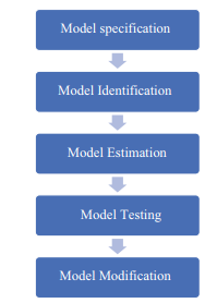
Fig. 3.1 Steps in SEM analysis

The structural model is specified when the latent construct in the measurement model is aptly measured by the observed variable as measurement model does not specify the directional relationship between the latent variables. The structural model specifies the relationship between latent variables in theoretical form. It is obvious that such relationship should be specified before estimation and testing of the model. The structural equation obtained evaluates the specific structure coefficient. Each equation has a prediction error which specifies the degree of variance in the latent endogenous variables. The equation also specifies the pre- dicted relationships. These relationships between latent and observed variables are also shown by the path diagram.

2. Model Identification: This is the second step in SEM analysis and happens prior to the estimation of model parameters which is the relationship between the vari- ables in the model. Model identification is concerned with the task of whether the unique solution can be formed for the model or not. It must theoretically establish unique estimate for each variable for the model to be Model identification is dependent on the parameters as free, fixed and constrained. Free parameters are those parameters which are unknown and which need to be esti- mated. Fixed parameters are those which are fixed at a specific value such as 0 or 1. Constrained parameters are those which are unknown but constrained to one or more other parameters. To identify the structural equation model, measure- ment model must be identified. The measurement model is identified in these two conditions. Firstly, there are two or more latent variables, each has at least three indicators loaded on it, and the errors of these variables are not It is also necessary that each indicator loads only one factor. Secondly, there are two or more latent variable, each has only two indicators loaded on it, and the error of these variables is not correlated. It is also necessary that each indicator loads only one factor, and variance or covariance among these factors is zero. A casual path from each latent variable to the observed variable should be zero for the likelihood of identification. Hence, reference variable is the variable which is fixed and non-zero loaded and has the most reliable scores.

A structural model to be identified could be extremely cumbersome and involves a highly complex calculation, and hence, structural model has to be outlined with a set of rules such as the recursive rule and t-rule. A structural model is said to be recursive when the model is unidirectional, i.e. when the two variables are related in only one directional. According to t-rule, the equation should have known pieces of information more than unknown pieces of information to determine a unique solution.

3. Model Estimation: The third step of the analysis is called model estimation. It estimates the theoretical model parameters in a way that the theoretical parameter values give a covariance matrix close to observed covariance matrix S. Structural modelling equation uses a iterative feature also known as fitting function. Fit- ting function is used to minimize the difference between the observed covariance matrix S and the estimated theoretical covariance matrix P, and hence, it improves the primary estimates of parameter with iterative calculation cycle. The final esti- mates give the best fit parameter to the observed covariance matrix S. Several estimation procedures are available such as least squares, maximum likelihood, asymptotic distribution free (ADF), unweighted least squares and generalized least squares. Maximum likelihood (ML) is most commonly used estimation technique which is followed by generalized least squares (GLS). Although ML and GLS are comparable to ordinary least squares (OLS) estimation used in multiple regression, they possess select key advantages over OLS estimation. In particular, ML and GLS are (a) not scale-dependent, (b) allow dichotomous exogenous variables and (c) offer consistent and asymptotically efficient results in large samples. ML and GLS assume multivariate normality of dependent vari- ables and are called full information techniques as they estimate all model param- eters simultaneously to produce a full estimation model. This is a key limitation with OLS. A use of asymptotically distribution-free (ADF) estimator is recom- mended when the assumption of multivariate normality is violated. ADF does not depend on the underlying distribution of the data, but it requires a large sam- ple size as the estimator yields inaccurate chi-square (χ ²) statistics for smaller sample sizes.

4. Model Testing: Structural equation modelling helps in concurrent analysis of both indirect and direct relationship among manifest and latent variables. The model testing includes the analysis of two conceptually distinct models such as structural and the measurement It is necessary for a researcher to ensure that the observed variable chosen for the latent variable is actual measure of construct. In absence of such verification, the structural model becomes mean- ingless. Model fitting has a problem that power varies with the sample size. For example, if we have a very huge sample size, then the sample test will always be significant, and hence, we reject the model, and on the other side, if we consider a very small sample, then model will always be accepted though it fits badly.

1. Model evaluation indices

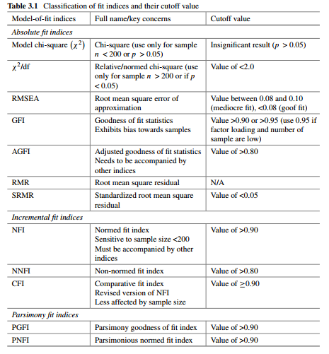
Evaluation of SEM is generally based on fit indices to test the single path coefficient such as p value and standard error and for the overall model such as χ², RMSEA. There are three types of model-of-fit indices:

• Absolute fit indices
• Incremental fit indices
• Parsimony fit indices (Fig 3.2).

2. Absolute fit indices

• It measures the overall goodness of fit for both the structural and measurement models collectively.
• Absolute fit indices are the indices which show that how well a priori model will be fitting in the sample data. It also shows that which model has the best superiority among the proposed models.

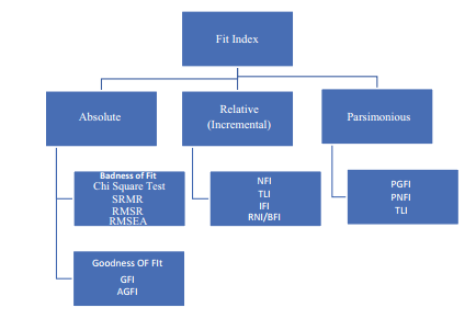
Fig. 3.2 Types of fit index

• The indices include the following: Models chi-square (χ²), relative/normed chi- square (χ²/df), RMSEA, GFI, AGFI, RMR and SRMR.

3. Incremental fit indices

• It is also known as comparative indices or relative fit indices.
• The indices include the following: NFI, NNFI and CFI.

4. Parsimony fit indices

• Estimation process is dependent on data when we have nearly saturated or complex model. Hence, we need less rigorous theoretical model that paradoxically gives better fit indices.
• The indices include the following: PGFI and PNFI (Table 3.1).

It is difficult to specify a generic guideline for fitness indices which can help the researcher to distinguish a good model from a poor model. However, the selected recommendations are outlined by Hair et al. (2012) include

• Goodness of the model should be verified using three to four indices of different types.
• Index cutoff values should be adjusted based on model characteristics.
• Employ the use of multiple indices to examine the goodness of the model. This helps the researcher to determine which model is better when the set of acceptable models are compared with the help of multiple indices.

5. Model Modification: This is the final step of structural equation A researcher intends to modify the model so that they explore the best-fitted model which fits the data perfectly. Firstly, researcher has to accomplish a model specification search which eliminates the non-significant parameters from the theoretical model which is also known as theory trimming, and then, they need to examine the model’s standardized residual matrix which is called as fitted residuals. To eliminate parameters, one common method is to compare the t– static for individual parameter to the tabled t-value to find its significance in the sample. While examining the standardized residual matrix, one should attempt to find all the values which are small in magnitude as large values in the matrix imply a misspecification of the general model, whereas large values across an individual variable imply to the misspecification in that individual variable only.

The above-said procedures can improve the fit of the model, but it is highly contradicted method as specification searches are exploratory in nature and thus are based on the sample data instead of previous theory and research, and as a result, parameter eliminated from the theoretical model may reflect sample characteristics that do not generalize to the broader population. Also, model modification may progress to an inflation of Type I error, and hence, it can be misleading. Therefore, it is recommended that a researcher should keep a balance while eliminating the parameters in the model to improve the fit of the model.

In summary, there are six steps in conducting structural equation modelling.

Step 1: Define the individual constructs. Typically, this should answer “what items to be used as measured varaibles?”

Step 2: Develop and specify the measurement model. This includes two things: (i) associate measured variables with constructs and (ii) develop a path diagram for the measurement model.

Step 3: Design a study to produce empirical results. Here, a researcher must exam- ine the adequacy of the sample size. In addition, he should select an appropriate estimation method and missing data approach.

Step 4: Assess the validty of measurement model. This should be done by examining goodness of fit (GOF) indices and construct validity of measurement model. If the mesurement model is valid as per the prescribed ranges of GOF and construct validity then a researcher can move to step 5. If this is not satisfied then a researcher must refine the measures and design a new study.

Step 5: Specify structural model. This requires measurement model to be converted into structural model by assigning relationships from one constructs to another based on the proposed theoretical model.

Step 6: Finally, a researcher should assess the validity of structural model by check- ing goodness of fit indices (GOF) and signficance, direction and size of structural parameters estimates. If the structural model is valid then researcher can draw sus- bstantive conclusions and extend necessary recommendations. If structural model fails the test of validity then a researcher should refine the model and test with new data set.

Source: Thakkar, J.J. (2020). “Procedural Steps in Structural Equation Modelling”. In: Structural Equation Modelling. Studies in Systems, Decision and Control, vol 285. Springer, Singapore.