Category: SEM-AMOS

Basic Concepts of Structural Equation Modeling

1. Latent versus Observed Variables

In the behavioral sciences, researchers are often interested in studying theoretical constructs that cannot be observed directly. These abstract phenomena are termed latent variables, or factors. Examples of latent variables in psychology are self-concept and motivation; in sociology, powerlessness and anomie; in education, verbal ability and teacher expectancy; in economics, capitalism and social class.

Because latent variables are not observed directly, it follows that they cannot be measured directly. Thus, the researcher must operationally define the latent variable of interest in terms of behavior believed to represent it. As such, the unobserved variable is linked to one that is observable, thereby making its measurement possible. Assessment of the behavior, then, constitutes the direct measurement of an observed variable, albeit the indirect measurement of an unobserved variable (i.e., the underlying construct). It is important to note that the term behavior is used here in the very broadest sense to include scores on a particular measuring instrument. Thus, observation may include, for example, self-report responses to an attitudinal scale, scores on an achievement test, in vivo observation scores representing some physical task or activity, coded responses to interview questions, and the like. These measured scores (i.e., measurements) are termed observed or manifest variables; within the context of SEM methodology, they serve as indicators of the underlying construct that they are presumed to represent. Given this necessary bridging process between observed variables and unobserved latent variables, it should now be clear why methodologists urge researchers to be circumspect in their selection of assessment measures. Although the choice of psychometrically sound instruments bears importantly on the credibility of all study findings, such selection becomes even more critical when the observed measure is presumed to represent an underlying construct.¹

2. Exogenous versus Endogenous Latent Variables

It is helpful in working with SEM models to distinguish between latent variables that are exogenous and those that are endogenous. Exogenous latent variables are synonymous with independent variables: they “cause” fluctuations in the values of other latent variables in the model. Changes in the values of exogenous variables are not explained by the model. Rather, they are considered to be influenced by other factors external to the model. Background variables such as gender, age, and socioeconomic status are examples of such external factors. Endogenous latent variables are synonymous with dependent variables and, as such, are influenced by the exogenous variables in the model, either directly or indirectly. Fluctuation in the values of endogenous variables is said to be explained by the model because all latent variables that influence them are included in the model specification.

3. The Factor Analytic Model

The oldest and best-known statistical procedure for investigating relations between sets of observed and latent variables is that of factor analysis. In using this approach to data analyses, the researcher examines the covariation among a set of observed variables in order to gather information on their underlying latent constructs (i.e., factors). There are two basic types of factor analyses: exploratory factor analysis (EFA) and confirmatory factor analysis (CFA). We turn now to a brief description of each.

Exploratory factor analysis (EFA) is designed for the situation where links between the observed and latent variables are unknown or uncertain. The analysis thus proceeds in an exploratory mode to determine how, and to what extent, the observed variables are linked to their underlying factors. Typically, the researcher wishes to identify the minimal number of factors that underlie (or account for) covariation among the observed variables. For example, suppose a researcher develops a new instrument designed to measure five facets of physical self-concept (e.g., Health, Sport Competence, Physical Appearance, Coordination, Body Strength). Following the formulation of questionnaire items designed to measure these five latent constructs, he or she would then conduct an EFA to determine the extent to which the item measurements (the observed variables) were related to the five latent constructs. In factor analysis, these relations are represented by factor loadings. The researcher would hope that items designed to measure Health, for example, exhibited high loadings on that factor, and low or negligible loadings on the other four factors. This factor analytic approach is considered to be exploratory in the sense that the researcher has no prior knowledge that the items do, indeed, measure the intended factors. (For texts dealing with EFA, see Comrey, 1992; Gorsuch, 1983; McDonald, 1985; Mulaik, 2009; for informative articles on EFA, see Byrne, 2005a; Fabrigar, Wegener, MacCallum, & Strahan, 1999; Floyd & Widaman, 1995; Preacher & MacCallum, 2003; MacCallum, Widaman, Zhang, & Hong, 1999; Wood, Tataryn, & Gorsuch, 1996.)

In contrast to EFA, confirmatory factor analysis (CFA) is appropriately used when the researcher has some knowledge of the underlying latent variable structure. Based on knowledge of the theory, empirical research, or both, he or she postulates relations between the observed measures and the underlying factors a priori and then tests this hypothesized structure statistically. For example, based on the example cited earlier, the researcher would argue for the loading of items designed to measure Sport Competence self-concept on that specific factor, and not on the Health, Physical Appearance, Coordination, or Body Strength self-concept dimensions. Accordingly, a priori specification of the CFA model would allow all Sport Competence self-concept items to be free to load on that factor, but restricted to have zero loadings on the remaining factors. The model would then be evaluated by statistical means to determine the adequacy of its goodness-of-fit to the sample data. (For texts dealing with CFA, see Brown, 2006; Mulaik, 2009; for detailed discussions of CFA, see, e.g., Bollen, 1989a; Byrne, 2003; Byrne, 2005b; Byrne, 2015; Long, 1983a.)

In summary, then, the factor analytic model (EFA or CFA) focuses solely on how, and the extent to which, the observed variables are linked to their underlying latent factors. More specifically, it is concerned with the extent to which the observed variables are generated by the underlying latent constructs and thus strength of the regression paths from the factors to the observed variables (i.e., the factor loadings) are of primary interest. Although inter-factor relations are also of interest, any regression structure among them is not considered in the factor analytic model. Because the CFA model focuses solely on the link between factors and their measured variables, within the framework of SEM, it represents what has been termed a measurement model.

4. The Full Latent Variable Model

In contrast to the factor analytic model, the full latent variable (LV) model allows for the specification of regression structure among the latent variables. That is to say, the researcher can hypothesize the impact of one latent construct on another in the modeling of causal direction. This model is termed “full” (or “complete”) because it comprises both a measurement model and a structural model: the measurement model depicting the links between the latent variables and their observed measures (i.e., the CFA model), and the structural model depicting the links among the latent variables themselves.

A full LV model that specifies direction of cause from one direction only is termed a recursive model; one that allows for reciprocal or feedback effects is termed a nonrecursive model. Only applications of recursive models are considered in the present book.

5. General Purpose and Process of Statistical Modeling

Statistical models provide an efficient and convenient way of describing the latent structure underlying a set of observed variables. Expressed either diagrammatically or mathematically via a set of equations, such models explain how the observed and latent variables are related to one another.

Typically, a researcher postulates a statistical model based on his or her knowledge of the related theory, on empirical research in the area of study, or some combination of both. Once the model is specified, the researcher then tests its plausibility based on sample data that comprise all observed variables in the model. The primary task in this model-testing procedure is to determine the goodness-of-fit between the hypothesized model and the sample data. As such, the researcher imposes the structure of the hypothesized model on the sample data, and then tests how well the observed data fit this restricted structure. Because it is highly unlikely that a perfect fit will exist between the observed data and the hypothesized model, there will necessarily be a differential between the two; this differential is termed the residual. The model-fitting process can therefore be summarized as follows:

Data = Model + Residual

where

Data represent score measurements related to the observed variables as derived from persons comprising the sample

Model represents the hypothesized structure linking the observed variables to the latent variables, and in some models, linking particular latent variables to one another

Residual represents the discrepancy between the hypothesized model and the observed data

In summarizing the general strategic framework for testing structural equation models, Joreskog (1993) distinguished among three scenarios, which he termed strictly confirmatory (SC), alternative models (AM), and model generating (MG). In the strictly confirmatory scenario, the researcher postulates a single model based on theory, collects the appropriate data, and then tests the fit of the hypothesized model to the sample data. From the results of this test, the researcher either rejects or fails to reject the model; no further modifications to the model are made. In the alternative models case, the researcher proposes several alternative (i.e., competing) models, all of which are grounded in theory. Following analysis of a single set of empirical data, he or she selects one model as most appropriate in representing the sample data. Finally, the model generating scenario represents the case where the researcher, having postulated and rejected a theoretically derived model on the basis of its poor fit to the sample data, proceeds in an exploratory (rather than confirmatory) fashion to modify and reestimate the model. The primary focus, in this instance, is to locate the source of misfit in the model and to determine a model that better describes the sample data. Joreskog (1993) noted that, although respecification may be either theory or data driven, the ultimate objective is to find a model that is both substantively meaningful and statistically well-fitting. He further posited that despite the fact that “a model is tested in each round, the whole approach is model generating, rather than model testing” (Joreskog, 1993, p. 295).

Of course, even a cursory review of the empirical literature will clearly show the MG situation to be the most common of the three scenarios, and for good reason. Given the many costs associated with the collection of data, it would be a rare researcher indeed who could afford to terminate his or her research on the basis of a rejected hypothesized model! As a consequence, the SC case is not commonly found in practice. Although the AM approach to modeling has also been a relatively uncommon practice, at least two important papers on the topic (e.g., MacCallum, Roznowski, & Necowitz, 1992; MacCallum, Wegener, Uchino, & Fabrigar, 1993) have precipitated more activity with respect to this analytic strategy.

Statistical theory related to these model-fitting processes can be found (a) in texts devoted to the topic of SEM (e.g., Bollen, 1989a; Kline, 2011; Loehlin, 1992; Long, 1983b; Raykov & Marcoulides, 2000; Saris & Stronkhurst, 1984; Schumacker & Lomax, 2004); (b) in edited books devoted to the topic (e.g., Bollen & Long, 1993; Cudeck, du Toit, & Sorbom, 2001; Hoyle, 1995a; Marcoulides & Schumacker, 1996); and (c) in methodologically oriented journals such as British Journal of Mathematical and Statistical Psychology, Journal of Educational and Behavioral Statistics, Multivariate Behavioral Research, Psychological Assessment, Psychological Methods, Psychometrika, Sociological Methodology, Sociological Methods & Research, and Structural Equation Modeling.

Source: Byrne Barbara M. (2016), Structural Equation Modeling with Amos: Basic Concepts, Applications, and Programming, Routledge; 3rd edition.

The General Structural Equation Model

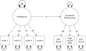
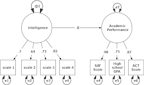
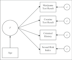
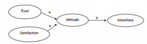
1. Symbol Notation

Structural equation models are schematically portrayed using particular configurations of four geometric symbols—a circle (or ellipse), a square (or rectangle), a single-headed arrow, and a double-headed arrow. By convention, circles (or ellipses; CD) represent unobserved latent factors, squares (or rectangles; ) represent observed variables, single-headed arrows (→) represent the impact of one variable on another, and double-headed arrows (^) represent covariances or correlations between pairs of variables. In building a model of a particular structure under study, researchers use these symbols within the framework of four basic configurations, each of which represents an important component in the analytic process. These configurations, each accompanied by a brief description, are as follows:

2. The Path Diagram

Schematic representations of models are termed path diagrams because they provide a visual portrayal of relations that are assumed to hold among the variables under study. Essentially, as you will see later, a path diagram depicting a particular SEM model is actually the graphical equivalent of its mathematical representation whereby a set of equations relates dependent variables to their explanatory variables. As a means of illustrating how the above four symbol configurations may represent a particular causal process, let me now walk you through the simple model shown in Figure 1.1, which was formulated using Amos Graphics (Arbuckle, 2015).

In reviewing the model shown in Figure 1.1, we see that there are two unobserved latent factors—math self-concept (MSC) and math achievement (MATH)—and five observed variables—three of which are considered to measure MSC (SDQMSC; APIMSC; SPPCMSC), and two to measure MATH (MATHGR; MATHACH). These five observed variables function as indicators of their respective underlying latent factors.

Associated with each observed variable is an error term (err1-err5), and with the factor being predicted (MATH), a residual term (resid1)²; there is an important distinction between the two. Error associated with observed variables represents measurement error, which reflects on their adequacy in measuring the related underlying factors (MSC; MATH). Measurement error derives from two sources: random measurement error (in the psychometric sense) and error uniqueness, a term used to describe error variance arising from some characteristic that is considered to be specific (or unique) to a particular indicator variable. Such error often represents nonrandom (or systematic) measurement error. Residual terms represent error in the prediction of endogenous factors from exogenous factors. For example, the residual term shown in Figure 1.1 represents error in the prediction of MATH (the endogenous factor) from MSC (the exogenous factor).

It is worth noting that both measurement and residual error terms, in essence, represent unobserved variables. Thus, it seems perfectly reasonable that, consistent with the representation of factors, they too should be enclosed in circles. For this reason, then, Amos path diagrams, unlike those associated with most other SEM programs, model these error variables as circled enclosures by default.

In addition to symbols that represent variables, certain others are used in path diagrams to denote hypothesized processes involving the entire system of variables. In particular, one-way arrows represent structural regression coefficients and thus indicate the impact of one variable on another. In Figure 1.1, for example, the unidirectional arrow pointing toward the endogenous factor, MATH, implies that the exogenous factor MSC (math self-concept) “causes” math achievement (MATH).⁴ Likewise, the three unidirectional arrows leading from MSC to each of the three observed variables (SDQMSC, APIMSC, SPPCMSC), and those leading from MATH to each of its indicators, MATHGR and MATHACH, suggest that these score values are each influenced by their respective underlying factors. As such, these path coefficients represent the magnitude of expected change in the observed variables for every change in the related latent variable (or factor). It is important to note that these observed variables typically represent subscale scores (see, e.g., Chapter 8), item scores (see, e.g., Chapter 4), item pairs (see, e.g., Chapter 3), and/or carefully formulated item parcels (see, e.g., Chapter 6).

The one-way arrows pointing from the enclosed error terms (err1-err5) indicate the impact of measurement error (random and unique) on the observed variables, and that from the residual (residl) indicates the impact of error in the prediction of MATH. Finally, as noted earlier, curved two-way arrows represent covariances or correlations between pairs of variables. Thus, the bidirectional arrow linking errl and err2, as shown in Figure 1.1, implies that measurement error associated with SDQMSC is correlated with that associated with APIMSC.

3. Structural Equations

As noted in the initial paragraph of this chapter, in addition to lending themselves to pictorial description via a schematic presentation of the causal processes under study, structural equation models can also be represented by a series of regression (i.e., structural) equations. Because (a) regression equations represent the influence of one or more variables on another, and (b) this influence, conventionally in SEM, is symbolized by a single-headed arrow pointing from the variable of influence to the variable of interest, we can think of each equation as summarizing the impact of all relevant variables in the model (observed and unobserved) on one specific variable (observed or unobserved). Thus, one relatively simple approach to formulating these equations is to note each variable that has one or more arrows pointing toward it, and then record the summation of all such influences for each of these dependent variables.

To illustrate this translation of regression processes into structural equations, let’s turn again to Figure 1.1. We can see that there are six variables with arrows pointing toward them; five represent observed variables (SDQMSC-SPPCMSC; MATHGR, MATHACH), and one represents an unobserved variable (or factor; MATH). Thus, we know that the regression functions symbolized in the model shown in Figure 1.1 can be summarized in terms of six separate equation-like representations of linear dependencies as follows:

MATH = MSC + resid1

SDQMSC = MSC + err1

APIMSC = MSC + err2

SPPCMSC = MSC + err3

MATHGR = MATH + err4

MATHACH = MATH + err5

4. Nonvisible Components of a Model

Although, in principle, there is a one-to-one correspondence between the schematic presentation of a model and its translation into a set of structural equations, it is important to note that neither of these model representations tells the whole story; some parameters critical to the estimation of the model are not explicitly shown and thus may not be obvious to the novice structural equation modeler. For example, in both the path diagram and the equations just shown, there is no indication that the variances of the exogenous variables are parameters in the model; indeed, such parameters are essential to all structural equation models. Although researchers must be mindful of this inadequacy of path diagrams in building model input files related to other SEM programs, Amos facilitates the specification process by automatically incorporating the estimation of variances by default for all independent factors.

Likewise, it is equally important to draw your attention to the specified nonexistence of certain parameters in a model. For example, in Figure 1.1, we detect no curved arrow between err4 and err5, which suggests the lack of covariance between the error terms associated with the observed variables MATHGR and MATHACH. Similarly, there is no hypothesized covariance between MSC and residl; absence of this path addresses the common, and most often necessary, assumption that the predictor (or exogenous) variable is in no way associated with any error arising from the prediction of the criterion (or endogenous) variable. In the case of both examples cited here, Amos, once again, makes it easy for the novice structural equation modeler by automatically assuming these specifications to be nonexistent. (These important default assumptions will be addressed in Chapter 2, where I review the specification of Amos models and input files in detail.)

5. Basic Composition

The general SEM model can be decomposed into two submodels: a measurement model and a structural model. The measurement model defines relations between the observed and unobserved variables. In other words, it provides the link between scores on a measuring instrument (i.e., the observed indicator variables) and the underlying constructs they are designed to measure (i.e., the unobserved latent variables). The measurement model, then, represents the CFA model described earlier in that it specifies the pattern by which each measure loads on a particular factor. In contrast, the structural model defines relations among the unobserved variables. Accordingly, it specifies the manner by which particular latent variables directly or indirectly influence (i.e., “cause”) changes in the values of certain other latent variables in the model.

For didactic purposes in clarifying this important aspect of SEM composition, let’s now examine Figure 1.2, in which the same model presented in Figure 1.1 has been demarcated into measurement and structural components.

Considered separately, the elements modeled within each rectangle in Figure 1.2 represent two CFA models. The enclosure of the two factors within the ellipse represents a full latent variable model and thus would not be of interest in CFA research. The CFA model to the left of the diagram represents a one-factor model (MSC) measured by three observed variables (SDQMSC-SPPCMSC), whereas the CFA model on the right represents a one-factor model (MATH) measured by two observed variables (MATHGR, MATHACH). In both cases, the regression of the observed variables on each factor and the variances of both the factor and the errors of measurement are of primary interest; the error covariance would be of interest only in analyses related to the CFA model bearing on MSC.

It is perhaps important to note that, although both CFA models described in Figure 1.2 represent first-order factor models, second- and higher-order CFA models can also be analyzed using Amos. Such hierarchical CFA models, however, are less commonly found in the literature (Kerlinger, 1984). Discussion and application of CFA models in the present book are limited to first- and second-order models only. (For a more comprehensive discussion and explanation of first- and second-order CFA models, see Bollen, 1989a; Brown, 2006; Kerlinger, 1984.)

6. The Formulation of Covariance and Mean Structures

The core parameters in structural equation models that focus on the analysis of covariance structures are the regression coefficients and the variances and covariances of the independent variables; when the focus extends to the analysis of mean structures, the means and intercepts also become central parameters in the model. However, given that sample data comprise observed scores only, there needs to be some internal mechanism whereby the data are transposed into parameters of the model. This task is accomplished via a mathematical model representing the entire system of variables. Such representation systems can, and do, vary with each SEM computer program. Because adequate explanation of the way in which the Amos representation system operates demands knowledge of the program’s underlying statistical theory, the topic goes beyond the aims and intent of the present volume. Thus, readers interested in a comprehensive explanation of this aspect of the analysis of covariance structures are referred to the following texts and monograph: Bollen (1989a), Saris & Stronkhorst (1984), Long (1983b).

In this chapter, I have presented you with a few of the basic concepts associated with SEM. As with any form of communication, one must first understand the language before being able to understand the message conveyed, and so it is in comprehending the specification of SEM models. Now that you are familiar with the basic concepts underlying structural equation modeling, we can turn our attention to the specification and analysis of models within the framework of the Amos program. In the next chapter, then, I provide you with details regarding the specification of models within the context of the program’s graphical interface as well as a new feature that allows for such specification in table (or spreadsheet) format. Along the way, I show you how to use the Toolbox facility in building models, review many of the drop-down menus, and detail specified and illustrated components of three basic SEM models. As you work your way through the applications included in this book, you will become increasingly more confident in both your understanding of SEM, and in using the Amos program. So, let’s move on to Chapter 2 and a more comprehensive look at SEM modeling with Amos.

Source: Byrne Barbara M. (2016), Structural Equation Modeling with Amos: Basic Concepts, Applications, and Programming, Routledge; 3rd edition.

Using the Amos Program

1. Key Concepts

Building SEM models using Amos Graphics
Building SEM models using Amos Tables View
Corollary associated with single variable estimation
Concept of model (or statistical) identification
Computing the number of degrees of freedom
Distinctions between first- and second-order CFA models
Changing Amos default color for constructed models

The program name, Amos, is actually an acronym for “Analysis of Moment Structures” or, in other words, the analysis of mean and covariance structures, the essence of SEM analyses. From Chapters 3 through 13, I walk you through use of the Amos program in the specification, testing, and interpretation of program output pertinent to a variety of confirmatory factor analytic (CFA) and path analytic models. However, before you can use any program in testing SEM models, it is essential that you first have a solid understanding of how to specify the model under test. In this regard, Amos differs from other SEM programs in that it provides you with a choice of four ways to specify models (described below). Only the graphical and recently developed tabular approaches will be illustrated throughout this volume. Based on a walk-through of three basic categories of SEM models, the intent of this chapter is to prepare you for the applications that follow by providing you with the necessary knowledge and technical skills needed in using these two approaches to model specification.

An interesting aspect of Amos is that, although developed within the Microsoft Windows interface and thus commonly considered to represent only a graphical approach to SEM, the program actually allows you to choose from four different modes of model specification. Using the Amos Graphics approach, you first build the model of interest and then work directly from this model in the conduct of various analyses. However, recognizing the fact that not everyone likes to work with graphics, Arbuckle (2012) recently (i.e., Version 21) introduced a Tables View¹ alternative. In lieu of building the model to be tested graphically, this option enables you to create exactly the same model, albeit using a spreadsheet approach. As such, all parameters of the model are listed in one of three or more tables each of which represents a common set of model components. Given that the Graphics and Tables View approaches to model specification represent two sides of the same coin, Arbuckle (2012) cleverly devised a tab on the Amos Graphics workspace that enables you to switch from one view to the other. For example, if you built the model graphically, then clicking on this tab would present you with the same model in Tables View format. Likewise, if you structured the model via Tables View, then a schematic representation of the equivalent model is just a click away. Lastly, the remaining two approaches, Amos VB.NET and Amos C#, enable you to work directly from equation statements. Regardless of which type of model specification you choose, all options related to the analyses are available from drop-down menus, and all estimates derived from the analyses can be presented in text format. In addition, however, Amos Graphics allows for the estimates to be displayed graphically in a path diagram.

The choice of which Amos method to use for model specification is purely arbitrary and really boils down to how comfortable you feel in working within either a graphical or table interface versus a more traditional programming interface. However, given the overwhelming popularity of the Amos Graphics approach to model specification by Amos users, together with the issue of space limitations, applications based on Amos VB.NET and/or Amos C# are not included in this volume. Nonetheless, for those who may be interested in using one or both of these approaches to model specification, detailed information can be accessed through the Amos Online Help option and many model examples can be found in the Amos User’s Guide (Arbuckle, 2015).

Throughout this third edition of the book, I focus primarily on the Amos Graphical approach to SEM, but include the equivalent Tables View representation of each model under study. Without a doubt, for those of you who enjoy working with draw programs, rest assured you will love working with Amos Graphics! All drawing tools have been carefully designed with SEM conventions in mind—and there is a wide array of them from which to choose. With a simple click of either the left or right mouse buttons, you will be amazed at how quickly you can build and specify an SEM model, run analyses in testing the model, and/or formulate a publication-quality path diagram.

In this chapter only, I walk you through the steps involved in the building of three example models based on Amos Graphics. In addition, given the newness of the Tables View format, I walk you through the same model specification process, albeit pertinent to the Example 1 only, using this table format option. So, let’s turn our attention first to a review of the various components and characteristics of Amos Graphics as they relate to the specification of three basic models—a first-order CFA model (Model 1), a second-order CFA model (Model 2), and a full SEM model (Model 3).

2. Model Specification Using Amos Graphics (Example 1)

To initiate Amos Graphics, you will need, first, to follow the usual Windows procedure as follows: Click on Start ^ All Programs ^ IBM SPSS Statistics ^ IBM SPSS Amos 23. As shown here, all work in this edition is based on Amos Version 23. Clicking on IBM SPSS Amos 23 presents the complete Amos selection listing. As shown in Figure 2.1, it is possible to access various files pertinent to previous work (e.g., data and model files, as well as other aspects of modeling in Amos). Initially, you will want to click on Amos Graphics. Alternatively, you can always place the Amos Graphics icon on your desktop.

Once you click on Amos Graphics, you will see the opening screen and toolbox shown in Figure 2.2. On the far right of this screen you will see a blank rectangle; this space provides for the drawing of your path diagram. The large highlighted icon at the top of the center section of the screen, when activated, presents you with a view of the input path diagram (i.e., the model specification). The companion icon to the right of the first one allows you to view the output path diagram; that is, the path diagram with the parameter estimates included. Of course, given that we have not yet conducted any analyses, this output icon is grayed out and not highlighted.

3. Amos Modeling Tools

Amos provides you with all the tools that you will ever need in creating and working with SEM path diagrams. Each tool is represented by an icon (or button) and performs one particular function; there are 42 icons from which to choose. As shown in Figure 2.2, the toolbox containing each of these icons is located on the far left of the palette. A brief description of each icon is presented in Table 2.1.

In reviewing Table 2.1, you will note that, although the majority of the icons are associated with individual components of the path diagram (e.g., |o]0), or with the path diagram as a whole (e.g., HU |Q]), others relate either to the data (e.g., H) or to the analyses (e.g., g]). Don’t worry about trying to remember this smorgasbord of tools, as simply holding the mouse pointer stationary over an icon is enough to trigger the pop-up label that identifies its function. As you begin working with Amos Graphics in drawing a model, you will find two tools, in particular, the Indicator icon [W] and the Error icon [g], to be worth their weight in gold! Both of these icons reduce, tremendously, the tedium of trying to align all multiple indicator variables, together with their related error variables in an effort to produce an aesthetically pleasing diagram. As a consequence, it is now possible to structure a path diagram in just a matter of minutes.

Now that you have had a chance to peruse the working tools of Amos Graphics, let’s move on to their actual use in formulating a path diagram. For your first experience in using this graphical interface, we’ll reconstruct the hypothesized CFA model shown in Figure 2.3.

4. The Hypothesized Model

The CFA structure in Figure 2.3 comprises four self-concept (SC) factors—academic SC (ASC), social SC (SSC), physical SC (PSC), and emotional SC (ESC). Each SC factor is measured by three observed variables, the reliability of which is influenced by random measurement error, as indicated by the associated error term. Each of these observed variables is regressed onto its respective factor. Finally, the four factors are shown to be intercorrelated.

5. Drawing the Path Diagram

To initiate the drawing of a new model, click on File shown at the top of the opening Amos screen and then select New from the drop-down menu. Although the File drop-down menu is typical of most Windows programs, I include it here in Figure 2.4 in the interest of completeness.

Now, we’re ready to draw our path diagram. The first tool you will want to use is, what I call, the “million dollar” (Indicator) icon (see Table 2.1) because it performs several functions. Click on this icon to activate it and then, with the cursor in the blank drawing space provided, hold down the left mouse button and draw an ellipse by dragging it slightly to create an ellipse shape.² If you prefer your factor model to show the factors as circles, rather than ellipses, just don’t perform the dragging action. When working with the icons, you need to release the mouse button after you have finished working with a particular function. Figure 2.5 illustrates the completed ellipse shape with the Indicator icon [*g] still activated. Of course, you could also have activated the Draw Unobserved Variables icon [£] and achieved the same result.

Now that we have the ellipse representing the first latent factor, the next step is to add the indicator variables. To do so, we click on the Indicator icon, after which the mouse pointer changes to resemble the Indicator icon. Now, move the Indicator icon image to the center of the ellipse at which time its outer rim becomes highlighted in red. Next, click on the unobserved variable. In viewing Figure 2.6, you will see that this action produces a rectangle (representing a single observed variable), an arrow pointing from the latent factor to the observed variable (representing a regression path), and a small circle with an arrow pointing toward the observed variable (representing a measurement error term).³ Again, you will see that the Indicator icon, when activated, appears in the center of the ellipse. This, of course, occurs because that’s where the cursor is pointing.

Note, however, that the hypothesized model (see Figure 2.3) we are endeavoring to structure schematically shows each of its latent factors to have three indicator variables, rather than only one. These additional indicators are easily added to the diagram by two simple clicks of the left mouse button while the Indicator icon is activated. In other words, with this icon activated, each time that the left mouse button is clicked, Amos Graphics will produce an additional indicator variable, each with its associated error term. Figures 2.7 and 2.8 show the results of having made one and two additional clicks, respectively, to the left mouse button.

In reviewing the hypothesized model again, we note that the three indicator variables for each latent factor are oriented to the left of the ellipse rather than to the top, as is currently the case in our diagram here. This task is easily accomplished by means of rotation. One very simple way of accomplishing this reorientation, is to click the right mouse button while the Indicator icon is activated. Figure 2.9 illustrates the outcome of this clicking action.

As you can see from the dialog box, there are a variety of options related to this path diagram from which you can choose. At this time, however, we are only interested in the Rotate option. Moving down the menu and clicking with the left mouse button on Rotate will activate the Rotate function and assign the related label to the cursor. When the cursor is moved to the center of the oval and the left mouse button clicked, the three indicator variables, in combination with their error terms and links to the underlying factor, will move 45 degrees clockwise as illustrated in Figure 2.10; two additional clicks will produce the desired orientation shown in Figure 2.11. Alternatively, we could have activated the Rotate icon [G] and then clicked on the ellipse to obtain the same effect.

Now that we have a one-factor structure completed, it becomes a simple task of duplicating this configuration in order to add three additional ones to the model. However, before we can duplicate, we must first group all components of this structure so that they operate as a single unit. This is easily accomplished by clicking on the Multiple Selection icon 0], after which you will observe that the outline of all factor structure components is now highlighted in blue, thereby indicating that they now operate as a unit. As with other drawing tasks in Amos, duplication of this structure can be accomplished either by clicking on the Duplicate icon [§], or by right-clicking on the model and activating the menu as shown in Figure 2.9. In both cases, you will see that with each click and drag of the left mouse button, the cursor takes on the form of a photocopier and generates one copy of the factor structure. This action is illustrated in Figure 2.12.

Once you have the number of copies that you need, it’s just a matter of dragging each duplicated structure into position. Figure 2.13 illustrates the four factor structures lined up vertically to replicate the hypothesized CFA model. Note the insert of the Move icon [™j in this figure. It is used to reposition objects from one location to another. In the present case, it was used to move the four duplicated factor structures such that they were aligned vertically. In composing your own SEM diagrams, you may wish to move an entire path diagram for better placement on a page. This realignment is made possible with the Move Icon, but don’t forget to activate the Select All icon illustrated first.⁴

Now we need to add the factor covariances to our path diagram. Illustrated in Figure 2.14 is the addition of a covariance between the first and fourth factors; these double-headed arrows are drawn by clicking on the Covariance icon 0. Once this button has been activated, you then click on one object (in this case, the first latent factor), and drag the arrow to the second object of interest (in this case, the fourth latent factor). The process is then repeated for each of the remaining specified covariances. Yes, gone are the days of spending endless hours trying to draw multiple arrows that look at least somewhat similar in their curvature! Thanks to Amos Graphics, these double-headed arrows are drawn perfectly every single time.

At this point, our path diagram, structurally speaking, is complete; all that is left to be done is to label each of the variables. If you look back at Figure 2.9, in which the mouse right-click menu is displayed, you will see a selection termed Object Properties at the top of the menu. This is the option you need in order to add text to a path diagram. To initiate this process, point the cursor at the object in need of the added text, right-click to bring up the View menu, and finally, left-click on Object Properties, which activates the dialog box shown in Figure 2.15. Of the five different tabs at the top of the dialog box, we select the Text tab, which then enables us to select a font size and style specific to the variable name to be entered. For purposes of illustration, I have simply entered the label for the first latent variable (ASC) and selected a font size of 12 with regular font style. All remaining labeling was completed in the same manner. Alternatively, you can display the list of variables in the data and then drag each variable to its respective rectangle.

The path diagram related to the hypothesized CFA model is now complete. However, before leaving Amos Graphics, I wish to show you the contents of four pull-down menus made available to you on your drawing screen. (For a review of a possible eight menus, see Figure 2.2.) The first and third drop-down menus (Edit; Diagram) shown in Figure 2.16 relate in some way to the construction of path diagrams. In reviewing these two menus, you will quickly see that they serve as alternatives to the use of drawing tools, some of which I have just demonstrated in the reconstruction of Figure 2.3. Thus, for those of you who may prefer to work with pull-down menus, rather than with drawing tool buttons, Amos Graphics provides you with this option. As its name implies, the View menu allows you to peruse various features associated with the variables and/or parameters in the path diagram. An important addition to this drop-down menu is the “Switch to Other View” option which, as noted earlier, was implemented in Version 21. As noted earlier regarding the tab on the Amos Graphics workspace, this option enables you to switch from a graphical view of a model to a parallel table view and vice versa. Finally, from the Analyze menu, you can calculate estimates (i.e., execute a job), manage groups and/or models, and conduct multiple group analyses as well as other types of analyses.

By now, you should have a fairly good understanding of how Amos Graphics works. Of course, because learning comes from doing, you will most assuredly want to practice some of the techniques illustrated here on your own.

For those of you who may still feel a little uncomfortable in working with the Amos Graphical approach to model building, I now walk you through the basic steps involved in specification of the same 4-factor model using the Tables View approach.

5. Model Specification Using Amos Tables View (Example 1)

As noted earlier, and as seen in Figure 2.2, the tab appearing at the base of the Amos work space enables you to build a model either as a path diagram using the graphical interface, or as a set of tables using the Tables View interface. Clicking on the “Path diagram” tab results in the blank worksheet shown in Figure 2.2.⁵ Alternatively, clicking on the “Tables” tab results in the work space shown in Figure 2.17. Closer examination of this space reveals three tables which, when used in combination, provide all the information needed in the specification of a CFA model. The first of these tables, labeled Variables, allows for identification of which variables are observed and which are not observed (i.e., latent). The next table, labeled Regression weights, provides information on which parameters (i.e., factor loadings and error variance terms) are fixed to 1.0 for purposes of model (or statistical) identification, a topic to be discussed immediately following this introduction to the Tables View interface. Finally, the third table, labeled Covariances, enables specification of which latent factors are hypothesized to covary with one another.

Let’s now walk through the process of specifying the 4-factor CFA model schematically displayed in Figure 2.3 using the Tables View approach.⁶^,⁷ Shown in Figure 2.18 are the three tables noted above, albeit with all specification information inserted in the appropriate cells. As such, the model, as specified in path analysis mode (Figure 2.3), is equivalent to Tables View mode (Figure 2.18). As I now explain the content of all table cells, I highly recommend that you have both Figures 2.3 and 2.18 in full view in order that you will fully comprehend the extent to which they are comparable to one another.

Let’s focus first on the first three lines of the Variables table in Figure 2.18. In the initial row, we see that the latent variable (ASC) has been entered, followed next by the first indicator variable (SDQASC1) associated with ASC, and finally, the error variance parameter associated with SDQASC1 (err1). Of these three parameters, only the SDQASC1 variable is observed

and, thus, the only one for which there is a checkmark appearing in the Observed column. The next four rows provide the same information, albeit related to the two additional indicator variables associated with ASC. Thus, the first seven rows of cells are pertinent only to Factor 1 of this model. Likewise, the next three sets of seven rows provide specification information for Factor 2 (SSC), Factor 3 (PSC, and Factor 4 (ESC).

Turning next to the Regression weights table, we see three columns labeled as “Dependent,” “Independent,” and “Parameter Name/Value.” In the first column, only the observed variables are listed, with each appearing on two consecutive rows. In all CFA models, the observed variables are always dependent variables in the model because, as shown in Figure 2.3, they have two sets of arrows (representing regression paths) pointing at them; the single-headed arrow leading from the latent variable to the observed variable represents the factor loading, and the one leading from the error term represents the impact of measurement error on the observed variable. Thus, for each line showing the same observed variable (e.g., SDQASC1), in column 2 you will see the two parameters on which it is regressed (e.g., ASC and errorl). This matching pattern is consistent for all observed variables in the model. Finally, in column 3, you will see a specification of “1”, but only for some of the entries in column 2. The reason for these entries of “1” is twofold. First, in a review of Figure 2.3, you will note that all regression paths leading from the error variances to the observed (or indicator) variables are shown with the numeral “1” above it, thereby signaling that these parameters are not estimated but, rather, are fixed to a value of “1”.

This specification addresses an important corollary in the modeling of single variables in SEM—you can estimate either the variance or the regression path, but you cannot estimate both. Because the error variance associated with each observed variable is of critical importance, its related error regression path is constrained to a fixed value of “1”. For this reason, then, error regression paths, by default, are automatically fixed to “1” in all SEM programs and this is the case here with respect to Amos. Thus, in reviewing these values in Column 3, you will see that the value of “1” is associated with all of the error terms. Second, turning again to Figure 2.3, you will note that the third indicator variable associated with each factor (e.g., SDQASC3 with ASC) is also fixed to “1”. Correspondingly, this value appears on the sixth line of the third column of the Regression weights table in Figure 2.18 as it relates to the same indicator/latent variable pairing; likewise for the three remaining factor loadings that have been constrained to “1” (SDQSSC3/ SSC; SDQPSC3/PSC; SDQESC/ESC). These fixed values address the issue of model (or statistical) identification, a topic to which we turn shortly.

Finally, in reviewing Figure 2.3 once again, you will note that the four latent factors are hypothesized to be intercorrelated as indicated by the double-headed arrows joining them. Turning to the table in Figure 2.18, it is easy to see that these same latent variable links are specified in table form via Columns 1 and 2.

In specifying a model using Tables View, I wish to pass along a few hints that I hope you will find helpful:

The sudden appearance of a red circle with an exclamation mark in its center serves as notification that something is wrong in a particular row. Running the mouse over this circle will yield the error message; typically, the problem is that you have inserted the same information in one of the other cells.
I purposefully entered information into the cells consistent with the labeling of the model in Figure 2.3 in order to keep things simple here. That is, I started at the top of the model with ASC and its related indicator variables. However, this type of ordering is not necessary. Rather, as long as you keep the same groupings together (e.g., ASC and its indicator variables), the order in which they are entered doesn’t matter (J. Arbuckle, personal communication, February 4,2014).
It can be difficult to alter the ordering of the regression weights once they have been entered. One workable solution is to completely delete the originally entered regression weight and then enter it again, albeit with the new regression weight value. Important to know here, however, is that the new weight will be added at the bottom of the list and the initial value should automatically be deleted from program memory (J. Arbuckle, personal communication, February 5, 2014).

As noted at the beginning of this journey into building models via the Tables View option, a single click of the dual Path diagram/Tables tab at the bottom of the Amos work space (see Figure 2.2 and 2.17) enables the user to easily switch between the two options. Given that we have now completed our specification of the CFA shown in Figure 2.3, no doubt you are expecting to see an exact replication of this figure once you click on the Path diagram tab. Thus, I’m sure it will be with some degree of shock that you view the model as completed in table format! Indeed, Figure 2.19 reveals exactly what you will see. Although the various components of the model look to be very random, this is not exactly the case. It’s just that in the process of adding each of the components to the model, Amos tries to prevent the circles and squares from overlapping, as well as to keep the arrows fairly short.

It is important to note that there is no need to reconstruct these elements to resemble the model in Figure 2.3. Even though the assemblage might look like a complete mess, rest assured that Amos knows all components of the model, as well as the specification of their related parameters. Thus, despite the rather disheveled-looking figure that you find upon completing the tables, all subsequent analyses remain the same as if you had built the model graphically. However, should you prefer to rearrange the components into the appropriate model, you can easily accomplish this task by working with selected draw tools from the toolbox. Likely the most valuable tool for this operation is the Move icon, introduced earlier in this chapter. Here, Figure 2.20 illustrates the beginning of this reconstruction process whereby the first indicator variable (SDQASC1) has been selected and moved to the top of the work page. Following the moving of several more of the indicator variables, latent factors, and single-headed and double-headed arrows, Figure 2.21 enables you to see the gradual formation of our 4-factor model of interest.

Now that you have been introduced to use of both the Amos Graphics and Tables View approaches to model specification, let’s move forward and examine our example Model 1 (see Figure 2.3) in more detail. We begin by studying the model’s basic components, default specification of particular parameters by the Amos program, and the critically important concept of model (or statistical) identification.

6. Understanding the Basic Components of Model 1

Recall from Chapter 1 that the key parameters to be estimated in a CFA model are the regression coefficients (i.e., factor loadings), the latent factor and error variances, and in some models (as is the case with Figure 2.3) the factor covariances. Given that the latent and observed variables are specified in the model in Amos Graphics (and in its Tables View alternative), the program automatically estimates the factor and error variances. In other words, variances associated with these specified variables are freely estimated by default. However, defaults related to parameter covariances, using Amos, are governed by the WYSIWYG rule—What You See Is What You Get. That is, if a covariance path is not included in the path diagram (or the matching table format), then this parameter will not be estimated (by default); if it is included, then its value will be estimated.

One extremely important caveat in working with structural equation models is to always tally the number of parameters in the model being estimated prior to running the analyses. This information is critical to your knowledge of whether or not the model that you are testing is statistically identified. Thus, as a prerequisite to the discussion of identification, let’s count the number of parameters to be estimated for the model portrayed in Figure 2.3. From a review of the figure, we can ascertain that there are 12 regression coefficients (factor loadings), 16 variances (12 error variances and 4 factor variances), and 6 factor covariances. The 1s assigned to one of each set of regression path parameters represent a fixed value of 1.00; as such, these parameters are not estimated. In total, then, there are 30 parameters to be estimated for the CFA model depicted in Figure 2.3. Let’s now turn to a brief discussion of the critically important concept of model (or statistical) identification.

7. The Concept of Model Identification

Model identification is a complex topic that is difficult to explain in nontechnical terms. Although a thorough explanation of the identification principle exceeds the scope of the present book, it is not critical to the reader’s understanding and use of Amos in the conduct of SEM analyses. Nonetheless, because some insight into the general concept of the identification issue will undoubtedly help you to better understand why, for example, particular parameters are specified as having values fixed to say, 1.00, I attempt now to give you a brief, nonmathematical explanation of the basic idea underlying this concept. Essentially, I address only the so-called “t-rule”, one of several tests associated with identification. I encourage you to consult the following texts for more comprehensive treatments of the topic: Bollen, 1989a; Kline, 2011; Long, 1983a, 1983b; Saris & Stronkhorst, 1984. I also highly recommend two book chapters having very clear and readable descriptions of the identification issue (Kenny & Milan, 2012; MacCallum, 1995), as well as an article addressing the related underlying assumptions (see Hayashi & Marcoulides, 2006).

In broad terms, the issue of identification focuses on whether or not there is a unique set of parameters consistent with the data. This question bears directly on the transposition of the variance-covariance matrix of observed variables (the data) into the structural parameters of the model under study. If a unique solution for the values of the structural parameters can be found, the model is considered to be identified. As a consequence, the parameters are considered to be estimable and the model therefore testable. If, on the other hand, a model cannot be identified, it indicates that the parameters are subject to arbitrariness, thereby implying that different parameter values define the same model; such being the case, attainment of consistent estimates for all parameters is not possible and, thus, the model cannot be evaluated empirically.

By way of a simple example, the process would be conceptually akin to trying to determine unique values for X and Y, when the only information you have is that X + Y = 15. Put another way, suppose that I ask you what two numbers add up to 15? You could say, for example, 10 + 5; 14 + 1; 8 + 7 and so on. In this instance, given that there are many ways by which you could attain the summation of 15, there is clearly no unique answer to the question. However, let’s say I ask you the same question but, instead, add that one of the numbers is 8; now you know exactly which number to select and therefore have a unique answer. Thus, by simply fixing the value of one number in the equation, you can immediately identify the missing number. Generalizing this simple example to SEM (also referred to as the analysis of covariance structures), the model identification issue focuses on the extent to which a unique set of values can be inferred for the unknown parameters from a given covariance matrix of analyzed variables that is reproduced by the model. Hopefully, this example also explains the basic rationale underlying the fixed value of 1.00 assigned to certain parameters in our specification of Model 1 in this chapter.

Structural models may be just-identified, overidentified, or underidentified. A just-identified model is one in which there is a one-to-one correspondence between the data and the structural parameters. That is to say, the number of data variances and covariances equals the number of parameters to be estimated. However, despite the capability of the model to yield a unique solution for all parameters, the just-identified model is not scientifically interesting because it has no degrees of freedom and therefore can never be rejected. An overidentified model is one in which the number of estimable parameters is less than the number of data points (i.e., variances and covariances of the observed variables). This situation

results in positive degrees of freedom that allow for rejection of the model, thereby rendering it of scientific use. The aim in SEM, then, is to specify a model such that it meets the criterion of overidentification. Finally, an underidentified model is one in which the number of parameters to be estimated exceeds the number of variances and covariances (i.e., data points). As such, the model contains insufficient information (from the input data) for the purpose of attaining a determinate solution of parameter estimation; that is, an infinite number of solutions are possible for an underidentified model.

Reviewing the CFA model in Figure 2.3, let’s now determine how many data points we have to work with (i.e., how much information do we have with respect to our data?). As noted above, these constitute the variances and covariances of the observed variables; with p variables, there are p(p + 1)/2 such elements. Given that there are 12 observed variables, this means that we have 12(12 + 1)/2 = 78 data points. Prior to this discussion of identification, we determined a total of 30 unknown parameters. Thus, with 78 data points and 30 parameters to be estimated, we have an overidentified model with 48 degrees of freedom.

However, it is important to note that the specification of an overidentified model is a necessary, but not a sufficient condition to resolve the identification problem. Indeed, the imposition of constraints on particular parameters can sometimes be beneficial in helping the researcher to attain an overidentified model. An example of such a constraint is illustrated in Chapter 5 with the application of a second-order CFA model.

Linked to the issue of identification is the requirement that every latent variable have its scale determined. This constraint arises because these variables are unobserved and therefore have no definite metric scale; it can be accomplished in one of two ways. The first approach is tied to specification of the measurement model, whereby the unmeasured latent variable is mapped onto its related observed indicator variable. This scaling requisite is satisfied by constraining to some nonzero value (typically 1.0), one factor loading parameter in each congeneric⁸ set of loadings. This constraint holds for both independent and dependent latent variables. In reviewing Figure 2.3, then, this means that for one of the three regression paths leading from each SC factor to a set of observed indicators, some fixed value should be specified; this fixed parameter is termed a reference variable.⁹ With respect to the model in Figure 2.3, for example, the scale has been established by constraining to a value of 1.0 the third parameter in each set of observed variables. Recall that in working through the Amos Graphical specification of Model 1, the program automatically assigned this value when the Indicator Variable icon was activated and used to add the first indicator variable and its error term to the model. Recall also, however, that these values were not added automatically with specification of the model using the table format. It is important to note that although Amos Graphics assigned the value of “1” to the lower regression path of each set, this assignment can be changed simply by clicking on the right mouse button and selecting Object Properties from the pop-up menu. (This modification will be illustrated with the next example.)

With a better idea of important aspects of the specification of a CFA model in general, specification using Amos (either the graphical or table format) in particular, as well as the basic notions associated with model identification, we now continue on our walk through the two remaining models reviewed in this chapter. As with Model 1, we begin by specifying Model 2 using the graphical approach to model specification.

8. Model Specification Using Amos Graphics (Example 2)

In this second example of model specification, we examine the second-order model displayed in Figure 2.22.

The Hypothesized Model

In our previous factor analytic model, we had four factors (ASC, SSC, PSC, ESC) which operated as independent variables; each could be considered to be one level, or one unidirectional arrow away from the observed variables. Such factors are termed first-order factors. However, it may be the case that the theory argues for some higher-level factor that is considered accountable for the lower-order factors. Basically, the number of levels or unidirectional arrows that the higher-order factor is removed from the observed variables determines whether a factor model is considered to be second-order, third-order, or some higher-order. Only a second-order model will be examined here.

Although the model schematically portrayed in Figure 2.22 has essentially the same first-order factor structure as the one shown in Figure 2.3, it differs in that a higher-order general self-concept (GSC) factor is hypothesized as accounting for, or explaining, all variance and covariance related to the first-order factors. As such, GSC is termed the second-order factor. It is important to take particular note of the fact that GSC does not have its own set of measured indicators; rather it is linked indirectly to those measuring the lower-order factors.

Let’s now take a closer look at the parameters to be estimated for this second-order model (Figure 2.22). First, note the presence of single-headed arrows leading from the second-order factor (GSC) to each of the first-order factors (ASC to ESC). These regression paths represent second-order factor loadings, and all are freely estimated. Recall, however, that for reasons linked to the model identification issue, a constraint must be placed either on one of the regression paths, or on the variance of an independent factor as these parameters cannot be estimated simultaneously. Because the impact of GSC on each of the lower-order SC factors is of primary interest in second-order CFA models, the variance of the higher-order factor is typically constrained to equal 1.0, thereby leaving the second-order factor loadings to be freely estimated.

A second aspect of this second-order model that perhaps requires some amplification is the initial appearance of the first-order factors operating as both independent and dependent variables. This situation is not so, however, as variables can serve either as independent or as dependent variables in a model, but not as both.¹⁰ Because the first-order factors function as dependent variables, it then follows that their variances and covariances are no longer estimable parameters in the model; such variation is presumed to be accounted for by the higher-order factor. In comparing Figures 2.3 and 2.22, then, you will note that there are no longer double-headed curved arrows linking the first-order SC factors, indicating that neither the factor covariances nor variances are to be estimated.

Finally, the prediction of each of the first-order factors from the second-order factor is presumed not to be without error. Thus, a residual error term is associated with each of the lower-level factors.

As a first step in determining whether this second-order model is identified we now sum the number of parameters to be estimated; we have 8 first-order regression coefficients, 4 second-order regression coefficients, 12 measurement error variances, and 4 residual error terms, making a total of 28. Given that there are 78 pieces of information in the sample variance-covariance matrix, we conclude that this model is identified with 50 degrees of freedom.

Before leaving this identification issue, however, a word of caution is in order. With complex models in which there may be more than one level of latent variable structures, it is wise to visually check each level separately for evidence that identification has been attained. For example, although we know from our initial CFA model that the first-order level is identified, it is quite possible that the second-order level may indeed be underidentified. Given that the first-order factors function as indicators of (i.e., the input data for) the second-order factor, identification is easy to assess. In the present model, we have four factors, giving us 10 (4 x 5/2) pieces of information from which to formulate the parameters of the higher-order structure. According to the model depicted in Figure 2.22, we wish to estimate 8 parameters (4 regression paths; 4 residual error variances), thus leaving us with 2 degrees of freedom, and an overidentified model. However, suppose that we only had three first-order factors. We would then be left with a just-identified model at the upper level as a consequence of trying to estimate 6 parameters from 6 (3[3 + 1])/2) pieces of information. In order for such a model to be tested, additional constraints would need to be imposed (see, e.g., Chapter 5). Finally, let’s suppose that there were only two first-order factors; we would then have an underidentified model since there would be only three pieces of information, albeit four parameters to be estimated. Although it might still be possible to test such a model, given further restrictions on the model, the researcher would be better advised to reformulate his or her model in light of this problem (see Rindskopf & Rose, 1988).

Drawing the Path Diagram

Now that we have dispensed with the necessary “heavy stuff,” let’s move on to creating the second-order model shown in Figure 2.22, which will serve as the specification input for Amos Graphics. We can make life easy for ourselves here simply by pulling up our first-order model (see Figure 2.3). Because the first-order level of our new model will remain the same as that shown in Figure 2.3, the only thing that needs to be done by way of modification is to remove all the factor covariance arrows. This task, of course, can be accomplished in Amos in one of two ways: either by activating the Erase icon [X] and clicking on each double-headed arrow, or by placing the cursor on each double-headed arrow individually and then right-clicking on the mouse, which produces the menu shown earlier.

Once you select the Erase option on the menu, the Erase icon will automatically activate and the cursor converts to a claw-like X symbol. Simply place the X over the component that you wish to delete and left-click; the targeted component disappears. As illustrated in Figure 2.23, the covariance between ASC and SSC has already been deleted with the covariance between ASC and PSC being the next one to be deleted. For both methods of erasure, Amos automatically highlights the selected parameter in red.

Having removed all the double-headed arrows representing the factor covariances from the model, our next task is to draw the ellipse representing the higher-order factor of GSC. We do this by activating the Draw Unobserved Variable icon [o], which, for me, resulted in an ellipse with solid red fill. However, for publication purposes, you will likely want the ellipse to be clear. To accomplish this, placing the cursor over the upper ellipse and right-clicking on the mouse again will produce a menu from which you select Object Properties. At this point, your model should resemble the one shown in Figure 2.24. Once in this dialog box, click on the Color tab, scroll down to Fill style, and then choose Transparent as illustrated in Figure 2.25. Note that you can elect to set this color option as default by clicking on the Set Default tab to the right.

Continuing with our path diagram, we now need to add the second-order factor regression paths. We accomplish this task by first activating the Path icon 0 and then, with the cursor clicked on the central underside of the GSC ellipse, dragging the cursor up to where it touches the central right side of the ASC ellipse. Figure 2.26 illustrates this drawing process with respect to the first path; the process is repeated for each of the other three paths.

Because each of the first-order factors is now a dependent variable in the model, we need to add the residual error term associated with the prediction of each by the higher-order factor of GSC. To do so, we activate the Error icon [g] and then click with the left mouse button on each of the ellipses representing the first-order factors. Figure 2.27 illustrates implementation of the residual error term for ASC. In this instance, only one click was completed, thereby leaving the residual error term in its current position (note the solid fill as I had not yet set the default for transparent fill). However, if we clicked again with the left mouse button, the error term would move 45 degrees clockwise as shown in Figure 2.28; with each subsequent click, the error term would continue to be moved clockwise in a similar manner.

The last task in completing our model is to label the higher-order factor, as well as each of the residual error terms. Recall that this process is accomplished by first placing the cursor on the object of interest (in this case the first residual error term) and then clicking with the right mouse button. This action releases the pop-up menu shown in Figure 2.24 from which we select Object Properties, which, in turn, yields the dialog box displayed in Figure 2.29. To label the first error term, we again select the Text tab and then add the text, res1; this process is then repeated for each of the remaining residual error terms.

9. Model Specification Using Amos Tables View (Example 2)

Let’s now view specification of this higher-order model from the Tables View perspective as presented in Figure 2.30. Turning first to the Variables table, you will note that, except for the last five rows (denoted by a side bracket), all specifications replicate those reported for the first-order model as shown in Figure 2.18. To fully comprehend the differences between the two model parameterizations, it is best to view both the model (Figure 2.22) and its matching tabled specifications (Figure 2.30) side by side. Note first that the higher-order factor GSC is now included and, in contrast to the other factors, has its variance fixed to a value of 1.00. This specification is then followed by the addition of four residual error terms, given that the four first-order factors are now dependent variables in the model.

Turning to the Regression weights table, you will see the addition of eight parameters, again singled out by a side bracket. Specification of the first-order factors (ASC, SSC, PSC, and ESC) in the first (Dependent) column, together with that of GSC in the second (Independent) column, represent the four higher-order factor loadings, which are freely estimated. The repeated specification of the first-order factors in Column 1, together with their related residual error terms in Column 2, with the latter showing fixed values of 1.00, represent the regression paths leading from each of the residuals to their respective factor.

Figure 2.30 Specification of the second-order model shown in Figure 2.22 as for-matted in the Tables View optional panel.

Finally, as shown in Figure 2.30, there are no covariance specifications. As noted earlier, this lack of specification results from the fact that in the specification of a second-order model, all covariation among the lower-order factors is accounted for by the higher-order factor, which is GSC in this instance.

Before moving on to our next model comprising Example 3, I wish to alert you to a couple of odd things that can happen in the building of models using both the Amos Graphics and Amos Tables View approaches. With respect to the Graphics approach, as noted earlier, the program—by default—constrains one of any congeneric set of indicator variables to 1.00. In my experience, I have found this default constraint to be typically specified for the last factor loading of any congeneric set.

Turning to the Tables View approach and to the Variables table in particular, you will note a different ordering of the factor loadings between Figure 2.18 and Figure 2.30. In the first figure, I input the variables beginning with the first variable comprising the congeneric set of three. However, in Figure 2.30, I allowed the program to complete the table, and as you can see, it began with the third variable comprising this congeneric set. I bring this to your attention as you may have queried the possibility of errors in the tables. However, this is not the case, and the analyses will proceed in the same manner, regardless of the order in which they are listed. For a similar situation, take a look now at the Regression weights table where you will observe the rather odd specification of the higher-order loading of ESC on GSC. In lieu of being included with the other three higher-order factor loadings, it appears by itself in the last row of the table.

Based solely on my own experience with these tables, I close out this work on Example 2 with the following caveat. I think it is best to avoid trying to re-order the specified values in either the Variables or Regression weights tables once they have been entered, as otherwise, you are likely to encounter a series of error messages advising that a value already exists for the parameter you are attempting to change. Alternatively, one corrective tactic that has been found to be effective is to just delete the problematic parameter or its related fixed value and simply add it again. You should then see that it has been added to the bottom of the list. Accordingly, Amos should forget the original position and remember the new position (J. Arbuckle, personal communication, February 5, 2014).

10. Model Specification Using Amos Graphics (Example 3)

For our last example, we’ll examine a full SEM model. Recall from Chapter 1 that, in contrast to a first-order CFA model, which comprises only a measurement component, and a second-order CFA model for which the higher-order level is represented by a reduced form of a structural model, the full structural equation model encompasses both a measurement and a structural model. Accordingly, the full model embodies a system of variables whereby latent factors are regressed on other factors as dictated by theory and/or empirical research, as well as on the appropriate observed measures. In other words, in the full SEM model, certain latent variables are connected by one-way arrows, the directionality of which reflects hypotheses bearing on the causal structure of variables in the model. We turn now to the hypothesized model.

The Hypothesized Model

For a clearer conceptualization of full SEM models, let’s examine the relatively simple structure presented in Figure 2.31. The structural component of this model represents the hypothesis that a child’s self-confidence (SCONF) derives from his or her self-perception of overall social competence (SSC; social SC) which, in turn, is influenced by the child’s perception of how well he or she gets along with family members (SSCF), as well as with his or her peers at school (SSCS). The measurement component of the model shows each of the SC factors to have three indicator measures, and the self-confidence factor to have two.

Turning first to the structural part of the model, we can see that there are four factors. The two independent factors (SSCF; SSCS) are postulated as being correlated with each other, as indicated by the curved two-way arrow joining them, but they are linked to the other two factors by a series of regression paths, as indicated by the unidirectional arrows. Because the factors SSC and SCONF have one-way arrows pointing at them, they are easily identified as dependent variables in the model. Residual errors associated with the regression of SSC on both SSCF and SSCS, and the regression of SCONF on SSC, are captured by the disturbance terms res1 and res2, respectively. Finally, because one path from each of the two independent factors (SSCF; SSCS) to their respective indicator variables is fixed to 1.0, their variances can be freely estimated; variances of the dependent variables (SSC; SCONF), however, are not parameters in the model.

By now, you likely feel fairly comfortable in interpreting the measurement portion of the model, and so, substantial elaboration is not necessary here. As usual, associated with each observed measure is an error term, the variance of which is of interest. (Because the observed measures technically operate as dependent variables in the model, as indicated by the arrows pointing toward them, their variances are not estimated.) Finally, to establish the scale for each unmeasured factor in the model (and for purposes of statistical identification), one parameter in each set of regression paths is fixed to 1.0; recall, however, that path selection for the imposition of this constraint was purely arbitrary.

For this, our last example, let’s again determine if we have an identified model. Given that we have 11 observed measures, we know that we have 66 (11[11 + 1]/2) pieces of information from which to derive the parameters of the model. Counting up the unknown parameters in the model, we see that we have 26 parameters to be estimated: 7 measurement regression paths; 3 structural regression paths; 2 factor variances; 11 error variances; 2 residual error variances; and 1 covariance. We therefore have 40 (66-26) degrees of freedom and, thus, an overidentified model.

Drawing the Path Diagram

Given what you now already know about drawing path diagrams within the framework of Amos Graphics, you likely would encounter no difficulty in reproducing the hypothesized model shown in Figure 2.31. Therefore, rather than walk you through the entire drawing process related to this model, I’ll take the opportunity here to demonstrate two additional features of the drawing tools that have either not yet been illustrated or illustrated only briefly. The first of these makes use of the Object Properties icon is] in reorienting the assignment of fixed “1” values that the program automatically assigns to the factor loading regression paths. Turning to Figure 2.31, focus on the SSCS factor in lower left corner of the diagram. Note that the fixed path for this factor has been assigned to the one associated with the prediction of QSSCS3. For purposes of illustration, let’s reassign the fixed value of “1” to the first regression path (QSSCS1). To carry out this reorientation process, we can either right-click on the mouse, or click on the Object Properties icon, which in either case activates the related dialog box; we focus here on the latter. In using this approach, we click first on the icon and then on the parameter of interest (QSSCS3 in this instance) which then results in the parameter value becoming enclosed in a broken line box (see Figure 2.32). Once in the dialog box, we click on the Parameter tab at the top, which then generates the dialog box shown in Figure 2.32. Note that the regression weight is listed as “1”. To remove this weight, we simply delete the value. To reassign this weight, we subsequently click on the first regression path (QSSCS1) and then on the Object Properties icon. This time, of course, the Object Properties dialog box indicates no regression weight (see Figure 2.33) and all we need to do is to add a value of “1” as shown in Figure 2.32 for indicator variable QSSCS3. Implementation of these last two actions yields a modified version of the originally hypothesized model (Figure 2.31), which is schematically portrayed in Figure 2.34.

The second feature I wish to demonstrate involves the reorientation of error terms, usually for purposes of improving the appearance of the path diagram. Although I briefly mentioned this procedure and showed the resulting reorientation with respect to Example 2, I consider it important to expand on my earlier illustration as it is a technique that comes in handy when you are working with path diagrams that may have many variables in the model. With the residual error terms in the 12 o’clock position, as in Figures 2.31 and 2.34, we’ll continue to click with the left mouse button until they reach the 10 o’clock position shown in Figure 2.35. Each click of the mouse results in a 45-degree clockwise move of the residual error term, with eight clicks thus returning us to the 12 o’clock position; the position indicated in Figure 2.35 resulted from seven clicks of the mouse.

Changing the Amos Default Color for Constructed Models

For some reason, which continues to remain a mystery to me, when you first create a figure in Amos Graphics, by program default, all components of the model are produced in a mauve/blue color. Of course, these colored models cannot be used for publication purposes. Thus, I need to show you how you can quite easily convert this default color to white (or any similar light color) of your preference.

Shown in Figure 2.36 is a simple model created in Amos Graphics and shown in the original defaulted color produced by the program. To begin the change of color, click on one ellipse or rectangle in the model and then right click to bring up the Object Properties dialog box. In my case here, I clicked on the MSC ellipse. Next, click on the Color tab and move the cursor down to the Fill color rectangle as shown in Figure 2.37. Clicking on Fill color opens to a dialog box showing two sets of color panels, which are shown in Figure 2.38. On the left, you can see where I have changed the color to white. You will also need to change the color in the second panel to white. As indicated in the second panel, you will need to keep scrolling down until you reach the color “White.”

Shown in Figure 2.39, you can see that the MSC ellipse is now white. Continuing on, the next step is to click on the Edit menu and then on Select All. You will see at this point, that every symbol in the figure is highlighted, indicating that all components have been selected. Click again on the Edit menu and then on Drag Properties, where you then put a checkmark next to the Colors square as shown in Figure 2.40. Ensure that only the Color square is checked. Next, drag the mouse pointer from the object for which you have changed the color (in this instance, the MSC ellipse) to any other ellipse or rectangle in the model. This action will result in the color of all remaining ellipses and rectangles becoming white as shown in Figure 2.41. Finally, click on Edit and then on Deselect All.

11. Model Specification Using Amos Tables View (Example 3)

Turning to the equivalent Tables View specification (see Figure 2.42) for this third example model (see Figure 2.31), you likely will have no difficulty in deciphering its hypothesized parameterization as most of the specifications resemble those explained for the two previous example models. However, let’s take a look at the Regression weights table. The completed cells for all variables down to, and including SCON2, should be recognizable as representing the fixed-1 values for one indicator variable
in each congeneric set, as well as for each of the error variance terms; these 1s, of course, represent their related regression paths; that is, the factor loading linking QSSCF1 to its related factor (SSCF) and the path leading from errl to the indicator variable QSSCF1.

Figure 2.42 Specification of the full structural equation model shown in Figure 2.31 as formatted in the Tables View optional panel.

For clarification, I have marked only the last five rows of the Regression weights table for further explanation. The first three of these rows relate to relations among SSCF, SSCS, SSC. As can be seen, SSC is regressed on the two constructs of SSCF and SSCS, both of which serve as predictors of SSC, but with some degree of error, which is captured by the error term (resl). The regression path associated with the error term resl, therefore calls for the specification of fixed value of 1. Likewise, the same explanation holds for specification of a fixed 1 for residual linked to SCONF (res2).

Finally, in the Covariance table, you will see the only factor covariance in this model, which is between SSCF and SSCS.

In Chapter 1, I introduced you to the basic concepts underlying SEM and, in the present chapter, extended this information to include brief explanations of the corollary bearing on specification of a single indicator variable, as well as the issue of model identification. In this chapter, specifically, I have endeavored to show you the Amos Graphics approach in specifying particular models under study, along with its related and newly incorporated Tables View approach. I hope that I have succeeded in giving you a fairly good idea of the ease by which Amos makes this process possible. Nonetheless, it is important for me to emphasize that, although I have introduced you to a wide variety of the program’s many features, I certainly have not exhausted the total range of possibilities, as to do so would far exceed the intended scope of the present book. Now that you are fairly well equipped with knowledge of the conceptual underpinning of SEM and the basic functioning of the Amos program, let’s move on to the remaining chapters where we explore the analytic processes involved in SEM using Amos Graphics. As noted earlier, for each of the chapters to follow, I will also include the equivalent Tables View specification format for each hypothesized and final model analyzed using Amos Graphics. We turn now to Chapter 3, which features an application bearing on a CFA model.

Source: Byrne Barbara M. (2016), Structural Equation Modeling with Amos: Basic Concepts, Applications, and Programming, Routledge; 3rd edition.

Application 1: Testing the Factorial Validity of a Theoretical Construct (First-Order CFA Model) with AMO

1. Key Concepts

Hypothesized models conceptualized within a matrix format
Error/uniqueness parameters
Congeneric measures
Working with model-refining tools in Amos Graphics
Specification of data in Amos Graphics
Calculation of estimates in Amos Graphics
Selection of textual versus graphical output in Amos Graphics
Evaluation of parameter estimates
Evaluation of model as a whole
model-fitting process
issue of statistical significance in SEM
estimation process
goodness-of-fit statistics
separate computation of standardized RMR
Issue of model misspecification
Use and interpretation of modification indices
Use and interpretation of standardized residuals
Calculation of standardized root mean square residual
Post hoc analyses: Justification versus no justification

Our first application examines a first-order CFA model designed to test the multidimensionality of a theoretical construct. Specifically, this application tests the hypothesis that self-concept (SC), for early adolescents (Grade 7), is a multidimensional construct composed of four factors—general SC (GSC), academic SC (ASC), English SC (ESC), and mathematics SC (MSC). The theoretical underpinning of this hypothesis derives from the hierarchical model of SC proposed by Shavelson, Hubner, and Stanton (1976). The example is taken from a study by Byrne and Worth Gavin (1996) in which four hypotheses related to the Shavelson et al. model were tested for three groups of children—preadolescents (Grade 3), early adolescents (Grade 7), and late adolescents (Grade 11). Only tests bearing on the multidimensional structure of SC, as they relate to grade 7 children, are of interest in the present chapter. This study followed from earlier work in which the same 4-factor structure of SC was tested for adolescents (see Byrne & Shavelson, 1986), and was part of a larger study that focused on the structure of social SC (Byrne & Shavelson, 1996). For a more extensive discussion of the substantive issues and the related findings, readers should refer to the original Byrne and Worth Gavin (1996) article.

2. The Hypothesized Model

At issue in this first application is the plausibility of a multidimensional SC structure for early adolescents. Although numerous studies have supported the multidimensionality of the construct for Grade 7 children, others have counter argued that SC is less differentiated for children in their pre- and early adolescent years (e.g., Harter, 1990). Thus, the argument could be made for a 2-factor structure comprising only GSC and ASC. Still others postulate that SC is a unidimensional structure so that all facets of SC are embodied within a single SC construct (GSC). (For a review of the literature related to these issues, see Byrne, 1996.) The task presented to us here, then, is to test the original hypothesis that SC is a 4-factor structure comprising a general domain (GSC), an academic domain (ASC), and two subject-specific domains (ESC; MSC), against two alternative hypotheses: (a) that SC is a 2-factor structure comprising GSC and ASC, and (b) that SC is a 1-factor structure in which there is no distinction between general and academic SCs.

We turn now to an examination and testing of each of these three hypotheses.

Hypothesis 1: Self-concept is a 4-Factor Structure

The model to be tested in Hypothesis 1 postulates a priori that SC is a 4-factor structure composed of general SC (GSC), academic SC (ASC), English SC (ESC), and math SC (MSC); it is presented schematically in Figure 3.1.

Prior to any discussion of how we might go about testing this model, let’s take a few minutes first to dissect the model and list its component parts as follows:

There are four SC factors, as indicated by the four ellipses labeled GSC, ASC, ESC, and MSC.
These four factors are intercorrelated, as indicated by the two-headed arrows.
There are 16 observed variables, as indicated by the 16 rectangles (SDQ2N01-SDQ2N43); they represent item-pairs from the General, Academic, Verbal, and Math SC subscales of the Self Description Questionnaire II (Marsh, 1992a).

The observed variables load on the factors in the following pattern: SDQ2N01-SDQ2N37) load on Factor 1; SDQ2N04-SDQ2N40 load on Factor 2; SDQ2N10-SDQ2N46 load on Factor 3; and SDQ2N07-SDQ2N42 load on Factor 4.
Each observed variable loads on one and only one factor.
Errors of measurement associated with each observed variable (err01-err43) are uncorrelated.

Summarizing these observations, we can now present a more formal description of our hypothesized model. As such, we state that the CFA model presented in Figure 3.1 hypothesizes a priori that

SC responses can be explained by four factors: GSC, ASC, ESC, and MSC.
Each item-pair measure has a nonzero loading on the SC factor that it was designed to measure (termed a “target loading”), and a zero-loading on all other factors (termed “nontarget loadings”).
The four SC factors, consistent with the theory, are correlated.
Error/uniquenesses¹ associated with each measure are uncorrelated.

Another way of conceptualizing the hypothesized model in Figure 3.1 is within a matrix framework as presented in Table 3.1. Thinking about the model components in this format can be very helpful because it is consistent with the manner in which the results from SEM analyses are commonly reported in program output files. Although Amos, as well as other Windows-based programs, also provides users with a graphical output, the labeled information is typically limited to the estimated values and their standard errors. The tabular representation of our model in Table 3.1 shows the pattern of parameters to be estimated within the framework of three matrices: the factor loading matrix, the factor variance/covariance matrix, and the error variance/ covariance matrix. For purposes of model identification and latent variable scaling (see Chapter 2), you will note that the first of each congeneric² set of SC measures in the factor loading matrix is set to 1.0; all other parameters are freely estimated (as represented by an asterisk [*]). Likewise, as indicated by the asterisks appearing in the variance/ covariance matrix, all parameters are to be freely estimated. Finally, in the error/uniqueness matrix, only the error variances are estimated; all error covariances are presumed to be zero.

3. Modeling with Amos Graphics

Provided with these two perspectives of the hypothesized model, let’s now move on to the actual testing of the model. We’ll begin by examining the route to model specification, data specification, and the calculation of parameter estimates within the framework of Amos Graphics.

Model Specification

The beauty of working with the Amos Graphics interface is that all we need to do is to provide the program with a hypothesized model; in the present case, we use the one portrayed in Figure 3.1. Given that I demonstrated most of the commonly-used drawing tools, and their application, in Chapter 2, there is no need for me to walk you through the construction of this model here. Likewise, construction of hypothesized models presented throughout the remainder of the book will not be detailed. Nonetheless, I take the opportunity, wherever possible, to illustrate a few of the other drawing tools or features of Amos Graphics not specifically demonstrated earlier. Accordingly, in the last two editions of this book, I noted two tools that, in combination, I had found to be invaluable in working on various parts of a model; these were the Magnification ]§] and the Scroll H tools. To use this approach in modifying graphics in a model, you first click on the Magnification icon, with each click enlarging the model slightly more than as shown in the previous view. Once you have achieved sufficient magnification, you then click on the Scroll icon to move around the entire diagram. Clicking on the Reduction tool SI would then return the diagram to the normal view. You can also zoom in on specific objects of a diagram by simply using the mouse wheel. Furthermore, the mouse wheel can also be used to adjust the magnification of the Loupe tool Although the Scroll tool enables you to move the entire path diagram around, you can also use the scrollbars that appear when the diagram extends beyond the Amos Graphics window. An example of magnification using the Loupe tool is presented in Figure 3.2. Finally, it is worth noting that when either the Scroll, Magnification, or Loupe tools are activated, a right-click of the mouse will provide a pop-up menu of different diagram features you may wish to access (see Figure 3.3).

Data Specification

Now that we have provided Amos with the model to be analyzed, our next job is to tell the program where to find the data. All data to be used in applications throughout this book have been placed in an Amos folder called “Data Files.” To activate this folder, we can either click on the Data File icon g§], or pull down the File menu and select “Data Files.” Either choice will trigger the Data Files dialog box displayed in Figure 3.4; it is shown here as it pops up in the forefront of your workspace.

In reviewing the upper section of this dialog box, you will see that the program has identified the Group Name as “Group number 1”; this labeling is default in the analysis of single sample data. The data file to be used for the current analysis is labeled “ASC7INDM.TXT,” and the sample size is 265; the 265/265 indicates that, of a total sample size of 265, 265 cases have been selected for inclusion in the analysis. In the lower half of the dialog box, you will note a View Data button that allows you to peruse the data in spreadsheet form should you wish to do so. Once you have selected the data file that will serve as the working file upon which your hypothesized model is based, you simply click the OK button.

In the example shown here, the selected data file was already visible in the Data Files dialog box. However, suppose that you needed to select this file from a list of several available data sets. To do so, you would click on the File Name button in the Data Files dialog box (see Figure 3.4). This action would then trigger the Open dialog box shown in Figure 3.5. Here, you select a data file and then click on the Open button. Once you have opened a file, it becomes the working file and its filename will then appear in the Data Files dialog box, as illustrated in Figure 3.4.

It is important that I point out some of the requirements of the Amos program in the use of external data sets. If your data files are in ASCII format, you may need to restructure them before you are able to conduct any analyses using Amos. Consistent with SPSS and many other Windows applications, Amos requires that data be structured in tab-delimited (as well as comma- or semicolon-delimited) text format. Thus, whereas the semicolon (rather than the comma) delimiter is used in many European and Asian countries, this is not a problem as Amos can detect which version of the program is running (e.g., French version) and then automatically defines a compatible delimiter. In addition, all data must reside in an external file. The data used in this chapter are in the form of a tab-delimited (.dat) text file. However, Amos supports several common database formats, including SPSS *.sav and Excel *.xl; I use all three text formatted data sets in this book.

Calculation of Estimates

Now that we have specified both the model to be analyzed and the data file upon which the analyses are to be based, all that is left for us to do is to execute the job; we do so by clicking on the Calculate Estimates icon H|. (Alternatively, we could select “Calculate Estimates” from the Analyze drop-down menu.) Once the analyses have been completed, Amos Graphics allows you to review the results from two different perspectives—graphical and textual. In the graphical output, all estimates are presented in the path diagram. These results are obtained by clicking on the View Output Path Diagram icon 0 found at the top of the middle section of the Amos main screen. Results related to the testing of our hypothesized model are presented in Figure 3.6, with the inserted values representing the nonstand- ardized estimates. To copy the graphical output to another file, such as a Word document, either click on the Duplication icon or pull down the Edit menu and select “Copy (to Clipboard).” You can then paste the output into the document.

Likewise, you have two methods of viewing the textual output—either by clicking on the Text Output icon m, or by selecting “Text Output” from the View drop-down menu. However, in either case, as soon as the analyses are completed, a red tab representing the Amos output file will appear on the bottom status bar of your computer screen. Let’s turn now to the output resulting from our test of the hypothesized model.

Amos Text Output: Hypothesized 4-Factor Model

Textual output pertinent to a particular model is presented very neatly in the form of summaries related to specific sections of the output file. This tree-like arrangement enables the user to select out sections of the output that are of particular interest. Figure 3.7 presents a view of this tree-like formation of summaries, with summary information related to the hypothesized 4-factor model open. To facilitate the presentation and discussion of results in this chapter, the material is divided into three primary sections: (a) Model Summary, (b) Model Variables and Parameters, and (c) Model Evaluation.

Model Summary

This very important summary provides you with a quick overview of the model, including the information needed in determining its identification status. Here we see that there are 136 distinct sample moments or, in other words, elements in the sample covariance matrix (i.e., number of pieces of information provided by the data), and 38 parameters to be estimated, leaving 98 degrees of freedom based on an overidentified model, and a chi-square value of 158.511 with probability level equal to .000.

Recall that the only data with which we have to work in SEM are the observed variables, which in the present case number 16. Based on the formula, p(p + 1)/2 (see Chapter 2), the sample covariance matrix for these data should yield 136 (16[17]/2) sample moments, which indeed, it does. A more specific breakdown of the estimated parameters is presented in the Model Variables and Parameters section discussed next. Likewise, an elaboration of the ML (maximum likelihood) chi-square statistic, together with substantially more information related to model fit, is presented and discussed in the Model Evaluation section.

Model Variables and Parameters

The initial information provided for the Amos text output file can be invaluable in helping you resolve any difficulties with the specification of a model. The first set of important information is contained in the output file labeled Variable Summary. As shown in Table 3.2, here you will find all the variables in the model (observed and latent), accompanied by their categorization as either observed or unobserved, and as endogenous or exogenous. Consistent with the model diagram in Figure 3.1, all the observed variables (i.e., the input data) operate as dependent (i.e., endogenous) variables in the model; all factors and error terms are unobserved, and operate as independent (i.e., exogenous) variables in the model. This information is followed by a summary of the total number of variables in the model, as well as the number in each of the four categories, shown in the boxed area in Table 3.2.

The next section of the output file, listed as Parameter Summary, focuses on a summary of the parameters in the model and is presented in Table 3.3. Moving from left to right by column, we see that there are 32 regression weights, 20 of which are fixed and 12 of which are estimated; the 20 fixed regression weights include the first of each set of 4 factor loadings and the 16 error terms. There are 6 covariances and 20 variances, all of which are estimated. In total, there are 58 parameters, 38 of which are to be estimated. Provided with this summary, it is now easy for you to determine the appropriate number of degrees of freedom and, ultimately, whether or not the model is identified. Although, of course this information is provided by the program as noted in Figure 3.7, it is always good (and fun?) to see if your calculations are consistent with those of the program.

Model Evaluation

Of primary interest in structural equation modeling is the extent to which a hypothesized model “fits” or, in other words, adequately describes the sample data. Given findings of an inadequate goodness-of-fit, the next logical step is to detect the source of misfit in the model. Ideally, evaluation of model fit should derive from a variety of perspectives and be based on several criteria that assess model fit from a diversity of perspectives. In particular, these evaluation criteria focus on the adequacy of (a) the parameter estimates, and (b) the model as a whole.

Parameter Estimates

In reviewing the model parameter estimates, three criteria are of interest: (a) the feasibility of the parameter estimates, (b) the appropriateness of the standard errors, and (c) the statistical significance of the parameter estimates. We turn now to a brief explanation of each.

Feasibility of parameter estimates. The initial step in assessing the fit of individual parameters in a model is to determine the viability of their estimated values. In particular, parameter estimates should exhibit the correct sign and size, and be consistent with the underlying theory. Any estimates falling outside the admissible range signal a clear indication that either the model is wrong or the input matrix lacks sufficient information. Examples of parameters exhibiting unreasonable estimates are correlations >1.00, negative variances, and covariance or correlation matrices that are not positive definite.

Appropriateness of standard errors. Standard errors reflect the precision with which a parameter has been estimated, with small values suggesting accurate estimation. Thus, another indicator of poor model fit is the presence of standard errors that are excessively large or small. For example, if a standard error approaches zero, the test statistic for its related parameter cannot be defined (Bentler, 2005). Likewise, standard errors that are extremely large indicate parameters that cannot be determined (Joreskog & Sorbom, 1993).³ Because standard errors are influenced by the units of measurement in observed and/or latent variables, as well as the magnitude of the parameter estimate itself, no definitive criterion of “small” and “large” has been established (see Joreskog & Sorbom, 1989).

Statistical significance of parameter estimates. The test statistic as reported in the Amos output is the critical ratio (C.R.), which represents the parameter estimate divided by its standard error; as such, it operates as a z-statistic in testing that the estimate is statistically different from zero. Based on a probability level of .05, then, the test statistic needs to be >±1.96 before the hypothesis (that the estimate equals 0.0) can be rejected. Nonsignificant parameters, with the exception of error variances, can be considered unimportant to the model; in the interest of scientific parsimony, albeit given an adequate sample size, they should be deleted from the model. On the other hand, it is important to note that nonsignificant parameters can be indicative of a sample size that is too small (K.G. Joreskog, personal communication, January, 1997).

Before we review this section of the Amos output, it is important to alert you that, by default, the program does not automatically include either the standardized parameter estimates or the modification indices (MIs; indicators of misfitting parameters in the model). This requested information must be conveyed to the program prior to proceeding with the calculation of the estimates. Because these additionally estimated values can be critically important in determining the adequacy of tested models, I requested this information prior to running the analyses under review here. To request this additional output information, you first either click on the Analysis Properties icon IHD, or select Analysis Properties from the View drop-down menu. Immediately upon clicking on Analysis Properties, you will be presented with the dialog box shown in Figure 3.8 in which the boxes associated with “Standardized estimates” and “Modification indices” have already been checked. Note, also, that I have entered the numeral 10 in the box representing the “Threshold for modification indices,” which I will explain later in my discussion of modification indices.

Let’s turn now to this section of the Amos output file. After selecting Estimates from the list of output sections (see Figure 3.7), you will be presented with the information shown in Table 3.4. As you can readily see, results are presented separately for the Factor Loadings (listed as Regression weights), the Covariances (in this case, for factors only), and the Variances (for both factors and measurement errors), with both the unstandardized and standardized estimates being reported. Parameter estimation information is presented very clearly and succinctly in the Amos text output file. Listed to the right of each parameter is its estimated value (Column 1), standard error (Column 2), critical ratio (Column 3), and probability value (Column 4). An examination of the unstandardized solution reveals all estimates to be reasonable, their standard errors to be low, and their critical ratios to be real, strong evidence of their strong statistical significance.

Model as a Whole

In the Model Summary presented in Figure 3.7, we observed that Amos provided the overall x² value, together with its degrees of freedom and probability value. However, this information is intended only as a quick overview of model fit. Indeed, the program, by default, provides many other fit statistics in its output file. Before turning to this section of the Amos output, however, it is essential that I first review four important aspects of fitting hypothesized models; these are (a) the model-fitting process, (b) the issue of statistical significance, (c) the estimation process, and (d) the goodness-of-fit statistics.

The model-fitting process. In Chapter 1, I presented a general description of this process and noted that the primary task is to determine goodness-of-fit between the hypothesized model and the sample data. In other words, the researcher specifies a model and then uses the sample data to test the model.

With a view to helping you gain a better understanding of the goodness-of-fit statistics presented in the Amos Output file, let’s take a few moments to recast this model-fitting process within a more formalized framework. For this, let S represent the sample covariance matrix (of observed variable scores), Z (sigma) represent the population covariance matrix, and 9 (theta) represent a vector that comprises the model parameters. Thus, Z(9) represents the restricted covariance matrix implied by the model (i.e., the specified structure of the hypothesized model). In SEM, the null hypothesis (H₀) being tested is that the postulated model holds in the population [i.e., Z = Z(9)]. In contrast to traditional statistical procedures, however, the researcher hopes not to reject H₀ (but see MacCallum, Browne, & Sugawara [1996] for proposed changes to this hypothesis-testing strategy).

The issue of statistical significance. The rationale underlying the practice of statistical significance testing has generated a plethora of criticism over, at least, the past four decades. Indeed, Cohen (1994) has noted that, despite Rozeboom’s (1960) admonition more than 55 years ago that “the statistical folkways of a more primitive past continue to dominate the local scene” (p. 417), this dubious practice still persists. (For an array of supportive, as well as opposing views with respect to this article, see the American Psychologist [1995], 50, 1098-1103.) In light of this historical bank of criticism, together with the current pressure by methodologists to cease this traditional ritual (see, e.g., Cohen, 1994; Kirk, 1996; Schmidt, 1996; Thompson, 1996), the Board of Scientific Affairs for the American Psychological Association recently appointed a task force to study the feasibility of phasing out the use of null hypothesis testing procedures, as described in course texts and reported in journal articles. Consequently, the end of statistical significance testing relative to traditional statistical methods may soon be a reality. (For a compendium of articles addressing this issue, see Harlow, Mulaik, & Steiger, 1997.)

Statistical significance testing with respect to the analysis of covariance structures, however, is somewhat different in that it is driven by degrees of freedom involving the number of elements in the sample covariance matrix and the number of parameters to be estimated. Nonetheless, it is interesting to note that many of the issues raised with respect to the traditional statistical methods (e.g., practical significance, importance of confidence intervals, importance of replication) have long been addressed in SEM applications. Indeed, it was this very issue of practical “nonsignificance” in model testing that led Bentler and Bonett (1980) to develop one of the first subjective indices of fit (the NFI); their work subsequently spawned the development of numerous additional practical indices of fit, many of which are included in the Amos output. Likewise, the early work of Steiger (1990; Steiger & Lind, 1980) precipitated the call for use of confidence intervals in the reporting of SEM findings (see, e.g., MacCallum et al., 1996). Finally, the classic paper by Cliff (1983) denouncing the proliferation of post hoc model fitting, and criticizing the apparent lack of concern for the dangers of overfitting models to trivial effects arising from capitalization on chance factors, spirited the development of evaluation indices (Browne & Cudeck, 1989; Cudeck & Browne, 1983), as well as a general call for increased use of cross-validation procedures (see, e.g., MacCallum et al., 1992,1994).

The estimation process. The primary focus of the estimation process in SEM is to yield parameter values such that the discrepancy (i.e., residual) between the sample covariance matrix S and the population covariance matrix implied by the model [Σ(θ)] is minimal. This objective is achieved by minimizing a discrepancy function, F[S, Σ(θ)], such that its minimal value (f_min) reflects the point in the estimation process where the discrepancy between S and Σ(θ) is least [S – Σ(θ) = minimum]. Taken together, then, F_min serves as a measure of the extent to which S differs from Σ(θ).

Goodness-of-fit statistics. Let’s now turn to the goodness-of-fit statistics that are presented in Table 3.5. This information, as for the parameter estimates, is taken directly from the Amos output. For each set of fit statistics, you will note three rows. The first row, as indicated, focuses on the Hypothesized model under test (i.e., Your Model), the second on the Saturated model, and the third on the Independence model. Explanation of the latter two models, I believe, is most easily understood within a comparative framework. As such, think of these three models as representing points on a continuum, with the Independence model at one extreme, the Saturated model at the other extreme, and the Hypothesized model somewhere in between. The Independence model is one of complete independence of all variables in the model (i.e., in which all correlations among variables are zero) and is the most restricted. In other words, it is a null model, with nothing going on here as each variable represents a factor. The Saturated model, on the other hand, is one in which the number of estimated parameters equals the number of data points (i.e., variances and covariances of the observed variables, as in the case of the just-identified model), and is the least restricted.

For didactic as well as space reasons, all goodness-of-fit statistics are provided only for the initially hypothesized model in this first application; for all remaining chapters, only those considered to be the most critical in EM analyses will be reported. We turn now to an examination of each cluster, as they relate to the Hypothesized model only. (Formulae related to each fit statistic can be found in Arbuckle, 2012.)

Focusing on the first set of fit statistics, we see the labels NPAR (number of parameters), CMIN (minimum discrepancy), DF (degrees of freedom), P (probability value), and CMIN/DF. The value of 158.511, under CMIN, represents the discrepancy between the unrestricted sample covariance matrix S, and the restricted covariance matrix 1(9) and, in essence, represents the Likelihood Ratio Test statistic, most commonly expressed as a chi-square (x²) statistic. It is important to note that, for the remainder of the book, I refer to CMIN as x². This statistic is equal to (N – 1)F_min (sample size minus 1, multiplied by the minimum fit function) and, in large samples, is distributed as a central x² with degrees of freedom equal to 1/2(p)(p + 1) – t, where p is the number of observed variables, and t is the number of parameters to be estimated (Bollen, 1989a). In general, H₀: Z = 1(8) is equivalent to the hypothesis that Z – Z(8) = 0; the x² test, then, simultaneously tests the extent to which all residuals in Z – Z(8) are zero (Bollen, 1989a). Framed a little differently, the null hypothesis (H₀) postulates that specification of the factor loadings, factor variances/covariances, and error variances for the model under study are valid; the x² test simultaneously tests the extent to which this specification is true. The probability value associated with x² represents the likelihood of obtaining a x² value that exceeds the x² value when H₀ is true. Thus, the higher the probability associated with x², the closer the fit between the hypothesized model (under H₀) and the perfect fit (Bollen, 1989a).

The test of our H₀, that SC is a 4-factor structure as depicted in Figure 3.1, yielded a x² value of 158.51, with 98 degrees of freedom and a probability of less than .0001 (p < .0001), suggesting that the fit of the data to the hypothesized model is not entirely adequate. Interpreted literally, this test statistic indicates that, given the present data, the hypothesis bearing on SC relations, as summarized in the model, represents an unlikely event (occurring less than one time in a thousand under the null hypothesis) and should be rejected.

However, both the sensitivity of the Likelihood Ratio Test to sample size and its basis on the central x² distribution, which assumes that the model fits perfectly in the population (i.e., that H₀ is correct), have led to problems of fit that are now widely known. Because the x² statistic equals (N – 1)F_min, this value tends to be substantial when the model does not hold and sample size is large (Joreskog & Sorbom, 1993). Yet, the analysis of covariance structures is grounded in large sample theory. As such, large samples are critical to the obtaining of precise parameter estimates, as well as to the tenability of asymptotic distributional approximations (MacCallum et al., 1996). Thus, findings of well-fitting hypothesized models, where the x² value approximates the degrees of freedom, have proven to be unrealistic in most SEM empirical research. More common are findings of a large x² relative to degrees of freedom, thereby indicating a need to modify the model in order to better fit the data (Joreskog & Sorbom, 1993). Thus, results related to the test of our hypothesized model are not unexpected. Indeed, given this problematic aspect of the Likelihood Ratio Test, and the fact that postulated models (no matter how good) can only ever fit real-world data approximately and never exactly, MacCallum et al. (1996) recently proposed changes to the traditional hypothesis-testing approach in covariance structure modeling. (For an extended discussion of these changes, readers are referred to MacCallum et al., 1996.)

Researchers have addressed the x² limitations by developing good- ness-of-fit indices that take a more pragmatic approach to the evaluation process. Indeed, the past three decades have witnessed a plethora of newly developed fit indices, as well as unique approaches to the modelfitting process (for reviews see, e.g., Gerbing & Anderson, 1993; Hu & Bentler, 1995; Marsh, Balla, & McDonald, 1988; Tanaka, 1993). One of the first fit statistics to address this problem was the x²/degrees of freedom ratio (Wheaton, Muthen, Alwin, & Summers, 1977) which appears as CMIN/DF, and is presented in the first cluster of statistics shown in Table 3.5.⁴ For the most part, the remainder of the Amos output file is devoted to these alternative indices of fit, and, where applicable, to their related confidence intervals. These criteria, commonly referred to as “subjective,” “practical,” or “ad hoc” indices of fit, are typically used as adjuncts to the x² statistic.

Turning now to the next group of statistics, we see the labels, RMR, GFI, AGFI, and PGFI. The Root Mean Square Residual (RMR) represents the average residual value derived from the fitting of the variance-covariance matrix for the hypothesized model I(9) to the variance-covariance matrix of the sample data (S). However, because these residuals are relative to the sizes of the observed variances and covariances, they are difficult to interpret. Thus, they are best interpreted in the metric of the correlation matrix (Hu & Bentler, 1995; Joreskog & Sorbom, 1989). The standardized RMR (SRMR), then, represents the average value across all standardized residuals, and ranges from zero to 1.00; in a well-fitting model this value will be small, say, .05 or less. The value of .103 shown in Table 3.5 represents the unstandardized residual value. Not shown on the output, however, is the SRMR value. Although this standardized coefficient is typically reported in the output file by other SEM programs, for some reason this is not the case with Amos. Nonetheless, this standardized value can be obtained in a three-step process. First, click on the tab labeled “Plug-ins” located at the top of the Amos Graphics opening page, which will then yield a drop-down menu where you will find “standardized RMR” as the last item listed. Second, click on “standardized RMR,” which then presents you with a blank screen. Finally, with the blank screen open, click on the “Calculate Estimates” icon. Once Amos has calculated this value it will appear in the blank screen. These three steps are shown in Figure 3.9, with the standardized RMR shown to be .0479. It can be interpreted as meaning that the model explains the correlations to within an average error of .048 (see Hu & Bentler, 1995).

The Goodness-of-fit Index (GFI) is a measure of the relative amount of variance and covariance in S that is jointly explained by I. The AGFI differs from the GFI only in the fact that it adjusts for the number of degrees of freedom in the specified model. As such, it also addresses the issue of parsimony by incorporating a penalty for the inclusion of additional parameters. The GFI and AGFI can be classified as absolute indices of fit because they basically compare the hypothesized model with no model at all (see Hu & Bentler, 1995). Although both indices range from zero to 1.00, with values close to 1.00 being indicative of good fit, Joreskog and Sorbom (1993) note that, theoretically, it is possible for them to be negative; Fan, Thompson, and Wang (1999) further caution that GFI and AGFI values can be overly influenced by sample size. This, of course, should not occur as it would reflect the fact that the model fits worse than no model at all.

Based on the GFI and AGFI values reported in Table 3.5 (.933 and .906, respectively) we can once again conclude that our hypothesized model fits the sample data fairly well.

The last index of fit in this group, the Parsimony Goodness-of-fit Index (PGFI), was introduced by James, Mulaik, and Brett (1982) to address the issue of parsimony in SEM. As the first of a series of “parsimony-based indices of fit” (see Williams & Holahan, 1994), the PGFI takes into account the complexity (i.e., number of estimated parameters) of the hypothesized model in the assessment of overall model fit. As such, “two logically interdependent pieces of information,” the goodness-of-fit of the model (as measured by the GFI) and the parsimony of the model, are represented by the single index PGFI, thereby providing a more realistic evaluation of the hypothesized model (Mulaik et al., 1989, p. 439). Typically, parsimony-based indices have lower values than the threshold level generally perceived as “acceptable” for other normed indices of fit. Mulaik et al. suggested that nonsignificant x² statistics and goodness-of-fit indices in the .90s, accompanied by parsimonious-fit indices in the 50s, are not unexpected. Thus, our finding of a PGFI value of .672 would seem to be consistent with our previous fit statistics.

We turn now to the next set of goodness-of-fit statistics (Baseline Comparisons), which can be classified as incremental or comparative indices of fit (Hu & Bentler, 1995; Marsh et al., 1988). As with the GFI and AGFI, incremental indices of fit are based on a comparison of the hypothesized model against some standard. However, whereas this standard represents no model at all for the GFI and AGFI, it represents a baseline model (typically the independence or null model noted above for the incremental indices).⁵ We now review these incremental indices.

For the better part of a decade, Bentler and Bonett’s (1980) Normed Fit Index (NFI) has been the practical criterion of choice, as evidenced in large part by the current “classic” status of its original paper (see Bentler, 1992; Bentler & Bonett, 1987). However, addressing evidence that the NFI has shown a tendency to underestimate fit in small samples, Bentler (1990) revised the NFI to take sample size into account and proposed the Comparative Fit Index (CFI; see last column). Values for both the NFI and CFI range from zero to 1.00 and are derived from the comparison of a hypothesized model with the independence (or null) model, as described earlier. As such, each provides a measure of complete covariation in the data, Although a value >.90 was originally considered representative of a well-fitting model (see Bentler, 1992), a revised cutoff value close to .95 has recently been advised (Hu & Bentler, 1999). Both indices of fit are reported in the Amos output; however, Bentler (1990) has suggested that, of the two, the CFI should be the index of choice. As shown in Table 3.5, the CFI (.962) indicated that the model fitted the data well in the sense that the hypothesized model adequately described the sample data. In somewhat less glowing terms, the NFI value suggested that model fit was only marginally adequate (.907). The Relative Fit Index (RFI; Bollen, 1986) represents a derivative of the NFI; as with both the NFI and CFI, the RFI coefficient values range from zero to 1.00, with values close to .95 indicating superior fit (see Hu & Bentler, 1999). The Incremental Index of Fit (IFI) was developed by Bollen (1989b) to address the issues of parsimony and sample size which were known to be associated with the NFI. As such, its computation is basically the same as the NFI, with the exception that degrees of freedom are taken into account. Thus, it is not surprising that our finding of IFI of .962 is consistent with that of the CFI in reflecting a well-fitting model. Finally, the Tucker-Lewis Index (TLI; Tucker & Lewis, 1973), consistent with the other indices noted here, yields values ranging from zero to 1.00, with values close to .95 (for large samples) being indicative of good fit (see Hu & Bentler, 1999).

The next cluster of fit indices all relate to the issue of model parsimony. The first fit index (PRATIO) relates to the initial parsimony ratio proposed by James et al. (1982). More appropriately, however, the index has subsequently been tied to other goodness-of-fit indices (see, e.g., the PGFI noted earlier). Here, it is computed relative to the NFI and CFI. In both cases, as was true for PGFI, the complexity of the model is taken into account in the assessment of model fit (see James et al., 1982; Mulaik et al., 1989). Again, a PNFI of .740 and PCFI of .785 (see Table 3.5) fall in the range of expected values.⁶

The next set of fit statistics provides us with the Noncentrality parameter (NCP) estimate. In our initial discussion of the x² statistic, we focused on the extent to which the model was tenable and could not be rejected. Now, however, let’s look a little more closely at what happens when the hypothesized model is incorrect [i.e., Z * Z(9)]. In this circumstance, the x² statistic has a noncentral x² distribution, with a noncentrality parameter, A, that is estimated by the noncentrality parameter (Bollen, 1989a; Hu & Bentler, 1995; Satorra & Saris, 1985). The noncentrality parameter is a fixed parameter with associated degrees of freedom, and can be denoted as x²(_df,_A). Essentially, it functions as a measure of the discrepancy between I and 1(0) and, thus, can be regarded as a “population badness-of-fit” (Steiger, 1990). As such, the greater the discrepancy between I and I(0), the larger the A value. (For a presentation of the various types of error associated with discrepancies among matrices, see Browne & Cudeck, 1993; Cudeck & Henly, 1991; MacCallum et al., 1994.) It is now easy to see that the central x² statistic is a special case of the noncentral x² distribution when A = 0.0. (For an excellent discussion and graphic portrayal of differences between the central and noncentral x² statistics, see MacCallum et al., 1996.) As a means to establishing the precision of the noncentrality parameter estimate, Steiger (1990) has suggested that it be framed within the bounds of confidence intervals. Turning to Table 3.5, we find that our hypothesized model yielded a noncentrality parameter of 60.511. This value represents the x² value minus its degrees of freedom (158.51 – 98). The confidence interval indicates that we can be 90% confident that the population value of the noncentrality parameter (A) lies between 29.983 and 98.953.

For those who may wish to use this information, values related to the minimum discrepancy function (FMIN) and the population discrepancy (FO) are presented next. The columns labeled LO90 and HI90 contain the lower and upper limits, respectively, of a 90% confidence interval around FO.

The next set of fit statistics focus on the Root Mean Square Error of Approximation (RMSEA). Although this index, and the conceptual framework within which it is embedded, was first proposed by Steiger and Lind in 1980, it has only recently been recognized as one of the most informative criteria in covariance structure modeling. The RMSEA takes into account the error of approximation in the population and asks the question, “how well would the model, with unknown but optimally chosen parameter values, fit the population covariance matrix if it were available?” (Browne & Cudeck, 1993, pp. 137-8). This discrepancy, as measured by the RMSEA, is expressed per degree of freedom thus making it sensitive to the number of estimated parameters in the model (i.e., the complexity of the model); values less than .05 indicate good fit, and values as high as .08 represent reasonable errors of approximation in the population (Browne & Cudeck, 1993). MacCallum et al. (1996) have recently elaborated on these cutpoints and noted that RMSEA values ranging from .08 to .10 indicate mediocre fit, and those greater than .10 indicate poor fit. Although Hu and Bentler (1999) have suggested a value of .06 to be indicative of good fit between the hypothesized model and the observed data, they caution that, when sample size is small, the RMSEA (and TLI) tend to over-reject true population models (but see Fan et al., 1999, for comparisons with other indices of fit). Although these criteria are based solely on subjective judgment, and therefore cannot be regarded as infallible or correct, Browne and Cudeck (1993) and MacCallum et al. (1996) argue that they would appear to be more realistic than a requirement of exact fit, where RMSEA = 0.0. (For a generalization of the RMSEA to multiple independent samples, see Steiger, 1998.)

Overall, MacCallum and Austin (2000) have strongly recommended routine use of the RMSEA for at least three reasons: (a) it appears to be adequately sensitive to model misspecification (Hu & Bentler, 1998); (b) commonly used interpretative guidelines appear to yield appropriate conclusions regarding model quality (Hu & Bentler, 1998, 1999); and (c) it is possible to build confidence intervals around RMSEA values.

Addressing Steiger’s (1990) call for the use of confidence intervals to assess the precision of RMSEA estimates, Amos reports a 90% interval around the RMSEA value. In contrast to point estimates of model fit (which do not reflect the imprecision of the estimate), confidence intervals can yield this information, thereby providing the researcher with more assistance in the evaluation of model fit. Thus, MacCallum et al. (1996) strongly urge the use of confidence intervals in practice. Presented with a small RMSEA, albeit a wide confidence interval, a researcher would conclude that the estimated discrepancy value is quite imprecise, negating any possibility to determine accurately the degree of fit in the population. In contrast, a very narrow confidence interval would argue for good precision of the RMSEA value in reflecting model fit in the population (MacCallum et al., 1996).

In addition to reporting a confidence interval around the RMSEA value, Amos tests for the closeness of fit. That is, it tests the hypothesis that the RMSEA is “good” in the population (specifically, that it is <.05). Joreskog and Sorbom (1996a) have suggested that the p-value for this test should be >.50.

Turning to Table 3.5, we see that the RMSEA value for our hypothesized model is .048, with the 90% confidence interval ranging from .034 to .062 and the p-value for the test of closeness of fit equal to .562. Interpretation of the confidence interval indicates that we can be 90% confident that the true RMSEA value in the population will fall within the bounds of .034 and .062 which represents a good degree of precision. Given that (a) the RMSEA point estimate is <.05 (.048); (b) the upper bound of the 90% interval is .06, which is less than the value suggested by Browne and Cudeck (1993), albeit equal to the cutoff value proposed by Hu and Bentler (1999); and (c) the probability value associated with this test of close fit is >.50 (p = .562), we can conclude that the initially hypothesized model fits the data well.⁷

Before leaving this discussion of the RMSEA, it is important to note that confidence intervals can be influenced seriously by sample size, as well as model complexity (MacCallum et al., 1996). For example, if sample size is small and the number of estimated parameters is large, the confidence interval will be wide. Given a complex model (i.e., a large number of estimated parameters), a very large sample size would be required in order to obtain a reasonably narrow confidence interval. On the other hand, if the number of parameters is small, then the probability of obtaining a narrow confidence interval is high, even for samples of rather moderate size (MacCallum et al., 1996).

Let’s turn, now, to the next cluster of statistics. The first of these is Akaike’s (1987) Information Criterion (AIC), with Bozdogan’s (1987) consistent version of the AIC (CAIC) shown at the end of the row. Both criteria address the issue of parsimony in the assessment of model fit; as such, statistical goodness-of-fit, as well as number of estimated parameters, are taken into account. Bozdogan (1987), however, noted that the AIC carried a penalty only as it related to degrees of freedom (thereby reflecting the number of estimated parameters in the model), and not to sample size. Presented with factor analytic findings that revealed the AIC to yield asymptotically inconsistent estimates, he proposed the CAIC, which takes sample size into account (Bandalos, 1993). The AIC and CAIC are used in the comparison of two or more models with smaller values representing a better fit of the hypothesized model (Hu & Bentler, 1995). The AIC and CAIC indices also share the same conceptual framework; as such, they reflect the extent to which parameter estimates from the original sample will cross-validate in future samples (Bandalos, 1993). The Browne-Cudeck Criterion (BCC; Browne & Cudeck, 1989) and the Bayes Information Criterion (BIC; Schwarz, 1978; Raftery, 1993) operate in the same manner as the AIC and CAIC. The basic difference among these indices is that both the BCC and BIC impose greater penalties than either the AIC or CAIC for model complexity. Turning to the output once again, we see that in the case of all four of these fit indices, the fit statistics for the hypothesized model are substantially smaller than they are for either the independence or the saturated models.

The Expected Cross-Validation Index (ECVI) is central to the next cluster of fit statistics. The ECVI was proposed, initially, as a means of assessing, in a single sample, the likelihood that the model cross-validates across similar-sized samples from the same population (Browne & Cudeck, 1989). Specifically, it measures the discrepancy between the fitted covariance matrix in the analyzed sample, and the expected covariance matrix that would be obtained in another sample of equivalent size. Application of the ECVI assumes a comparison of models whereby an ECVI index is computed for each model and then all ECVI values are placed in rank order; the model having the smallest ECVI value exhibits the greatest potential for replication. Because ECVI coefficients can take on any value, there is no determined appropriate range of values.

In assessing our hypothesized 4-factor model, we compare its ECVI value of .888 with that of both the saturated model (ECVI = 1.030) and the independence model (ECVI = 6.548). Given the lower ECVI value for the hypothesized model, compared with both the independence and saturated models, we conclude that it represents the best fit to the data. Beyond this comparison, Browne and Cudeck (1993) have shown that it is now possible to take the precision of the estimated ECVI value into account through the formulation of confidence intervals. Turning to Table 3.5 again, we see that this interval ranges from .773 to 1.034. Taken together, these results suggest that the hypothesized model is well-fitting and represents a reasonable approximation to the population. The last fit statistic, the MECVI, is actually identical to the BCC, except for a scale factor (Arbuckle, 2015).

The last goodness-of-fit statistic appearing on the Amos output is Hoelter’s (1983) Critical N (CN) (albeit labeled as Hoelter’s .05 and .01 indices). This fit statistic differs substantially from those previously discussed in that it focuses directly on the adequacy of sample size, rather than on model fit. Development of Hoelter’s index arose from an attempt to find a fit index that is independent of sample size. Specifically, its purpose is to estimate a sample size that would be sufficient to yield an adequate model fit for a x² test (Hu & Bentler, 1995). Hoelter (1983) proposed that a value in excess of 200 is indicative of a model that adequately represents the sample data. As shown in Table 3.5, both the .05 and .01 CN values for our hypothesized SC model were >200 (204 and 223, respectively). Interpretation of this finding, then, leads us to conclude that the size of our sample (N = 265) was satisfactory according to Hoelter’s benchmark that the CN should exceed 200.

Having worked your way through this smorgasbord of goodness-of- fit measures, you are no doubt feeling totally overwhelmed and wondering what you do with all this information! Although you certainly don’t need to report the entire set of fit indices, such an array can give you a good sense of how well your model fits the sample data. But how does one choose which indices are appropriate in evaluating model fit? Unfortunately, this choice is not a simple one, largely because particular indices have been shown to operate somewhat differently given the sample size, estimation procedure, model complexity, and/or violation of the underlying assumptions of multivariate normality and variable independence. Thus, Hu and Bentler (1995) caution that, in choosing which goodness-of-fit indices to use in the assessment of model fit, careful consideration of these critical factors is essential. For further elaboration on the above goodness-of-fit statistics with respect to their formulae and functions, or the extent to which they are affected by sample size, estimation procedures, misspecification, and/or violations of assumptions, readers are referred to Arbuckle (2015); Bandalos (1993); Boomsma and Hoogland (2001); Beauducel and Wittmann (2005); Bentler and Yuan (1999); Bollen (1989a); Brosseau-Liard, Savalei, and Li (2014); Browne and Cudeck (1993); Curran, West, and Finch (1996); Davey, Savla, and Luo (2005); Fan et al. (1999); Fan and Sivo (2005); Finch, West, and MacKinnon (1997); Gerbing and Anderson (1993); Hu and Bentler (1995, 1998, 1999); Hu, Bentler, and Kano (1992); Joreskog and Sorbom (1993); La Du and

Tanaka (1989); Lei and Lomax (2005); Marsh et al. (1988); Mulaik et al. (1989); Raykov and Widaman (1995); Stoel, Garre, Dolan, and van den Wittenboer (2006); Sugawara and MacCallum (1993); Tomarken and Waller (2005); Weng and Cheng (1997); West, Finch, and Curran (1995); Wheaton (1987); Williams and Holahan (1994); for an annotated bibliography, see Austin and Calderon (1996).

In finalizing this section on model assessment, I wish to leave you with this important reminder—that global fit indices alone cannot possibly envelop all that needs to be known about a model in order to judge the adequacy of its fit to the sample data. As Sobel and Bohrnstedt (1985, p. 158) so cogently stated more than three decades ago, “Scientific progress could be impeded if fit coefficients (even appropriate ones) are used as the primary criterion for judging the adequacy of a model.” They further posited that, despite the problematic nature of the x² statistic, exclusive reliance on goodness-of-fit indices is unacceptable. Indeed, fit indices provide no guarantee whatsoever that a model is useful. In fact, it is entirely possible for a model to fit well and yet still be incorrectly specified (Wheaton, 1987). (For an excellent review of ways by which such a seemingly dichotomous event can happen, readers are referred to Bentler and Chou, 1987.) Fit indices yield information bearing only on the model’s lack of fit. More importantly, they can in no way reflect the extent to which the model is plausible; this judgment rests squarely on the shoulders of the researcher. Thus, assessment of model adequacy must be based on multiple criteria that take into account theoretical, statistical, and practical considerations.

Thus far, on the basis of our goodness-of-fit results, we could very well conclude that our hypothesized 4-factor CFA model fits the sample data well. However, in the interest of completeness, and for didactic purposes, I consider it instructive to walk you through the process involved in determining evidence of model misspecification. That is, we conduct an analysis of the data that serves in identifying any parameters that have been incorrectly specified. Let’s turn now to the process of determining evidence of model misspecification.

Model Misspecification

Although there are two types of information that can be helpful in detecting model misspecification—the modification indices and the standardized residuals—typically most researchers are interested in viewing the modification indices as they provide a more direct targeting of parameters that may be misspecified. For this reason, it is always helpful to have this information included in the analysis output. (Recall that I showed you earlier how to request this information via Analysis Properties.) We turn first to explanation regarding modification indices (MIs), and then to that for the residuals.

Modification indices. Information derived from MIs reflects the extent to which the hypothesized model is appropriately described. Should there be some indication of misspecification, such evidence is captured by the MIs, which can be conceptualized as a x² statistic with one degree of freedom (Joreskog & Sorbom, 1993). Specifically, for each fixed parameter specified in the model (e.g., nontarget loadings automatically fixed to 0.0), Amos provides an MI, the value of which represents the expected drop in overall x² value if the parameter were to be freely estimated in a subsequent run; all freely estimated parameters automatically have MI values equal to zero. Although this decrease in X² is expected to approximate the MI value, the actual differential can be larger. Associated with each MI is an Expected Parameter Change (EPC) value (Saris, Satorra, & Sorbom, 1987) which is reported in the accompanying column labeled Par Change. This latter statistic represents the predicted estimated change, in either a positive or negative direction, for each fixed parameter in the model and yields important information regarding the sensitivity of the evaluation of fit to any reparameterization of the model.⁸

As alluded to earlier in this chapter, MI values less than 10.00 are generally considered of little value as freely estimating a formerly fixed parameter on the basis of an MI less than 10.00 will not result in any significant change to overall model fit. For this reason, then, I changed the Amos default cutpoint value of 4 to that of 10. As a result, only parameters having MI values great than 10 appear in the output as shown in Figure 3.10.

As can be seen in Figure 3.10, there was only one MI that had a value greater than 10. It represented a possible covariance between the error variances related to the indicator variables of SDQ2N25 and SDQ2N01. The MI is shown to be 13.487 and the EPC value to be .285. Interpreted broadly, the MI value suggests that if this parameter were to be freely estimated in a subsequent analysis, the overall chi-square value would drop by approximately 13.487 and the estimated error covariance would take on an approximate value of .285. In essence, this change would not have made any substantial difference to the model fit at all. However, more details regarding the impact of MIs in decisions of whether or not to modify a model will be presented in the next chapter, as well as all remaining chapters.

For purposes of comparison, let’s look now at the output file you would have received had the MI cutpoint been left at the Amos default value of 4. As you will note, this information, presented in Table 3.6, contains MIs and EPC values related to error covariances and factor loadings (i.e., the regression weights). Recall that the only model parameters for which the MIs are applicable are those that were fixed to a value of 0.0. Thus, no values appear under the heading Variances as all parameters representing variances (factors and measurement errors) were freely estimated.

In reviewing the parameters in the Covariance section, the only ones that make any substantive sense are those representing error covariances. In this regard, only the parameter representing a covariance between err25 and err01, as noted in Figure 3.9, would appear to be of any interest. Nonetheless, as noted above, an MI value of this size (13.487), with an EPC value of .285, particularly as these values relate to an error covariance, can be considered of little concern. Turning to the Regression weights, I consider only two to make any substantive sense; these are SDQ2N07 ^ ESC, and SDQ2N34 ^ MSC. Both parameters represent cross-loadings (i.e., secondary loadings). Here again, however, the MIs, and their associated EPC values, are not worthy of inclusion in a subsequently specified model.

Residuals. Recall that the essence of SEM is to determine the fit between the restricted covariance matrix [1(9)], implied by the hypothesized model, and the sample covariance matrix (S); any discrepancy between the two is captured by the residual covariance matrix. Each element in this residual matrix, then, represents the discrepancy between the covariances in 1(9) and those in S [i.e., 1(9) – S]; that is to say, there is one residual for each pair of observed variables (Joreskog, 1993). In the case of our hypothesized model, for example, the residual matrix would contain [(16 x 17)/2] = 136 elements. It may be worth noting that, as in conventional regression analysis, the residuals are not independent of one another. Thus, any attempts to test them (in the strict statistical sense) would be inappropriate. In essence, only their magnitude is of interest in alerting the researcher to possible areas of model misfit.

The matrices of both unstandardized and standardized residuals are available for inclusion in Amos output simply by checking off the Residuals option in the Analysis Properties dialog box (see Figure 3.8).

However, because the fitted residuals are dependent on the unit of measurement of the observed variables, they can be difficult to interpret and thus their standardized values are typically examined. As such, only the latter are presented in Table 3.7. Standardized residuals are fitted residuals divided by their asymptotically (large sample) standard errors (Joreskog & Sorbom, 1993). As such, they are analogous to Z-scores and are therefore the easier of the two sets of residual values to interpret. In essence, they represent estimates of the number of standard deviations the observed residuals are from the zero residuals that would exist if model fit were perfect [i.e., Σ(θ) – S=0.0]. Values >2.58 are considered to be large (Joreskog & Sorbom, 1993). In examining the standardized residual values presented in Table 3.7, we observe only one that exceeds the cutpoint of 2.58. As such, the standardized residual value of -2.942 reflects on the covariance between the observed variables SDQ2N07 and SDQ2N34. Thus, we can conclude that the only statistically significant discrepancy of note here lies with the covariance between the two item pairs.

Of prime importance in determining whether or not to include additional parameters in a model is the extent to which (a) they are substantively meaningful, (b) the existing model exhibits adequate fit, and (c) the EPC value is substantial. Superimposed on this decision is the ever-constant need for scientific parsimony. Because model respecification is commonly conducted in SEM in general, as well as in several applications highlighted in this book, I consider it important to provide you with a brief overview of the various issues related to these post hoc analyses.

5. Post Hoc Analyses

In the application of SEM in testing for the validity of various hypothesized models, the researcher will be faced, at some point, with the decision of whether or not to respecify and reestimate the model. If he or she elects to follow this route, it is important to realize that analyses then become framed within an exploratory, rather than a confirmatory mode. In other words, once a hypothesized CFA model, for example, has been rejected, this spells the end of the confirmatory factor analytic approach, in its truest sense. Although CFA procedures continue to be used in any respecification and reestimation of the model, these analyses would then be considered to be exploratory in the sense that they focus on the detection of misfitting parameters in the originally hypothesized model. Such post hoc analyses are conventionally termed “specification searches” (see MacCallum, 1986). (The issue of post hoc model fitting is addressed further in Chapter 9 in the section dealing with cross-validation.)

The ultimate decision underscoring whether or not to proceed with a specification search is twofold. First and foremost, the researcher must determine whether the estimation of the targeted parameter is substantively meaningful. If, indeed, it makes no sound substantive sense to free up the parameter exhibiting the largest MI, then one may wish to consider the parameter having the next largest MI value (Joreskog, 1993). Second, one needs to consider whether or not the respecified model would lead to an overfitted model. The issue here is tied to the idea of knowing when to stop fitting the model, or as Wheaton (1987, p. 123) phrased the problem, “knowing… how much fit is enough without being too much fit.” In general, overfitting a model involves the specification of additional parameters in the model after having determined a criterion that reflects a minimally adequate fit. For example, an overfitted model can result from the inclusion of additional parameters that (a) are “fragile” in the sense of representing weak effects that are not likely replicable, (b) lead to a significant inflation of standard errors, and (c) influence primary parameters in the model, albeit their own substantive meaningfulness is somewhat equivocal (Wheaton, 1987). Although correlated errors often fall into this latter category,⁹ there are many situations—particularly with respect to social psychological research, where these parameters can make strong substantive sense and therefore should be included in the model (Joreskog & Sorbom, 1993).

Having laboriously worked our way through the process involved in evaluating the fit of a hypothesized model, what can we conclude regarding the CFA model under scrutiny in the present chapter? In answering this question, we must necessarily pool all the information gleaned from our study of the Amos output. Taking into account (a) the feasibility and statistical significance of all parameter estimates, (b) the substantially good fit of the model, with particular reference to the CFI (.962) and RMSEA (.048) values, and (c) the lack of any substantial evidence of model misfit, I conclude that any further incorporation of parameters into the model would result in an overfitted model. Indeed, MacCallum et al. (1992, p. 501) have cautioned that, “when an initial model fits well, it is probably unwise to modify it to achieve even better fit because modifications may simply be fitting small idiosyncratic characteristics of the sample.” Adhering to this caveat, I conclude that the 4-factor model schematically portrayed in Figure 3.1 represents an adequate description of self-concept structure for grade 7 adolescents.

6. Hypothesis 2: Self-concept is a 2-Factor Structure

The model to be tested here (Model 2) postulates a priori that SC is a 2-factor structure consisting of GSC and ASC. As such, it argues against the viability of subject-specific academic SC factors. As with the 4-factor model, the four GSC measures load onto the GSC factor; in contrast, all other measures load onto the ASC factor. This hypothesized model is represented schematically in Figure 3.11, which serves as the model specification for Amos Graphics.

In reviewing the graphical specification of Model 2, two points pertinent to its modification are of interest. First, while the pattern of factor loadings remains the same for the GSC and ASC measures, it changes for both the ESC and MSC measures in allowing them to load onto the ASC factor. Second, because only one of these eight ASC factor loadings needs to be fixed to 1.0, the two previously constrained parameters (SDQ2N10 ^ ESC; SDQ2N07 ^ MSC) are now freely estimated.

Selected Amos Text Output: Hypothesized 2-Factor Model

Only the goodness-of-fit statistics are relevant to the present application, and a selected group of these is presented in Table 3.8.

As indicated in the output, the x²(W3) value of 455.926 represents an extremely poor fit to the data, and a substantial decrement from the overall fit of the 4-factor model (A x²(₅)=297.415). The gain of five degrees of freedom can be explained by the estimation of two fewer factor variances and five fewer factor covariances, albeit the estimation of two additional factor loadings (formerly SDQ2N10 ^ ESC and SDQ2N07 ^ MSC). As expected, all other indices of fit reflect the fact that self-concept structure is not well represented by the hypothesized 2-factor model. In particular, the CFI value of .776 and RMSEA value of .114, together with a PCLOSE value of 0.00 are strongly indicative of inferior goodness-of-fit between the hypothesized 2-factor model and the sample data. Finally, the ECVI value of 1.977, compared with the substantially lower value of 0.888 for the hypothesized 4-factor model again confirms the inferior fit of Model 2.

7. Hypothesis 3: Self-concept is a 1-Factor Structure

Although it now seems obvious that the structure of SC for grade 7 adolescents is best represented by a multidimensional SC structure, there are still researchers who contend that SC is a unidimensional construct. Thus, for purposes of completeness, and to address the issue of unidimensionality, Byrne and Worth Gavin (1996) proceeded in testing the above hypothesis. However, because the 1-factor model represents a restricted version of the 2-factor model, and thus cannot possibly represent a better-fitting model, in the interest of space, these analyses are not presented here.

In summary, it is evident from these analyses that both the 2-factor and 1-factor models of self-concept represent a misspecification of factorial structure for early adolescents. Based on these findings, then, Byrne and Worth Gavin (1996) concluded that SC is a multidimensional construct, which in their study comprised the four facets of general, academic, English, and math self-concepts.

8. Modeling with Amos Tables View

Thus far in this chapter, I have walked you through both the specification and testing of hypothesized models using the Amos Graphics approach. In order to provide you with two perspectives of specifications for the same model, let’s now view the hypothesized 4-factor model (Model 1) within the framework of the Amos Tables View format, which is captured in Figure 3.12. Turning first to the Variables table, you will readily note that the only boxes checked are those associated with an item as they represent the only observed variables in the data. In contrast, the constructs of GSC, ASC, ESC, and MSC as latent factors, together with the error terms, represent unobserved variables. Looking next at the Regression weights table, we see a “1” associated with each of the error variances. As you know from Chapter 2, this value of 1.00 indicates that the regression path linking the error term with its associated observed variable (the item) is fixed to a value of 1.00 and is therefore not estimated. Finally, the Covariances table reveals that the four factors are hypothesized to covary with one another.

In this first application, testing of the models was fairly straightforward and lacked any additional complexity as a result of the analyses. As a consequence, I was able to present the entire set of Tables in Figure 3.12. However, in the chapters that follow, the models become increasingly complex and thus, due to limitations of space in the writing of a book such as this one, some portions of the Tables View output may need to be eliminated as I zero-in on particular areas of interest. Nevertheless, given that you have full access to the datasets used in this book, I urge you to conduct the same analyses, at which time you will be able to view the entire output.

Source: Byrne Barbara M. (2016), Structural Equation Modeling with Amos: Basic Concepts, Applications, and Programming, Routledge; 3rd edition.

Application 2: Testing the Factorial Validity of Scores from a Measurement Scale (First-Order CFA Model) with AMOS

1. Key Concepts

Assumption of multivariate normality
The issue of multivariate outliers
The issue of multivariate kurtosis
Statistical strategies in addressing nonnormality
SEM robust statistics
Post hoc model testing and related issues
Nested models and the chi-square difference test
Error covariances and related issues

2. Modeling with Amos Graphics

For our second application, we once again examine a first-order confirmatory factor analysis (CFA) model. However, this time we test hypotheses bearing on a single measuring instrument, the Maslach Burnout Inventory (MBI; Maslach & Jackson, 1981, 1986), designed to measure three dimensions of burnout, which the authors label Emotional Exhaustion (EE), Depersonalization (DP), and Reduced Personal Accomplishment (PA). The term “burnout” denotes the inability to function effectively in one’s job as a consequence of prolonged and extensive job-related stress; “emotional exhaustion” represents feelings of fatigue that develop as one’s energies become drained, “depersonalization” – the development of negative and uncaring attitudes toward others, and “reduced personal accomplishment” – a deterioration of self-confidence, and dissatisfaction in one’s achievements.

Purposes of the original study (Byrne, 1994a), from which this example is taken, were to test for the validity and invariance of factorial structure within and across gender for elementary and secondary teachers. More specifically, the intent of the study was threefold: (a) to test for the factorial validity of the MBI separately for male/female elementary and secondary teachers, (b) to cross-validate findings across a second independent sample for each of these populations, and (c) to test for invariant factorial measurement and structure across gender for each of the two teaching panels. For the purposes of this chapter, however, only analyses bearing on the factorial validity of the MBI for a calibration sample of elementary male teachers (n = 372) are of interest.

Confirmatory factor analysis of a measuring instrument is most appropriately applied to measures that have been fully developed and their factor structures validated. The legitimacy of CFA use, of course, is tied to its conceptual rationale as a hypothesis-testing approach to data analysis. That is to say, based on theory, empirical research, or a combination of both, the researcher postulates a model and then tests for its validity given the sample data. Thus, application of CFA procedures to assessment instruments that are still in the initial stages of development represents a serious misuse of this analytic strategy. In testing for the validity of factorial structure for an assessment measure, the researcher seeks to determine the extent to which items designed to measure a particular factor (i.e., latent construct) actually do so. In general, subscales of a measuring instrument are considered to represent the factors; all items comprising a particular subscale are therefore expected to load onto their related factor.

Given that the MBI has been commercially marketed since 1981, is the most widely used measure of occupational burnout, and has undergone substantial testing of its psychometric properties over the years (see e.g., Byrne 1991, 1993, 1994b), it most certainly qualifies as a candidate for CFA research. Interestingly, until my 1991 study of the MBI, virtually all previous factor analytic work had been based only on exploratory procedures. We turn now to a description of this assessment instrument.

The Measuring Instrument under Study

The MBI is a 22-item instrument structured on a 7-point Likert-type scale that ranges from 0, “feeling has never been experienced,” to 6, “feeling experienced daily.” It is composed of three subscales, each measuring one facet of burnout; the EE subscale comprises nine items, the DP subscale five, and the PA subscale eight. The original version of the MBI (Maslach & Jackson, 1981) was constructed from data based on samples of workers from a wide range of human service organizations. Subsequently, however, Maslach and Jackson (1986), in collaboration with Schwab, developed the Educators’ Survey (MBI Form Ed), a version of the instrument specifically designed for use with teachers. The

MBI Form Ed parallels the original version of the MBI except for the modified wording of certain items to make them more appropriate to a teacher’s work environment.

3. The Hypothesized Model

The CFA model of MBI structure hypothesizes a priori that (a) responses to the MBI can be explained by three factors—EE, DP, and PA; (b) each item has a nonzero loading on the burnout factor it was designed to measure, and zero loadings on all other factors; (c) the three factors are correlated; and (d) the error/uniqueness terms associated with the item measurements are uncorrelated. A schematic representation of this model is shown in Figure 4.I.¹

This hypothesized 3-factor model of MBI structure provides the Amos Graphics specifications for the model to be tested here. In Chapter 2, we reviewed the process involved in computing the number of degrees of freedom and, ultimately, in determining the identification status of a hypothesized model. Although all such information (estimated/fixed parameters; degrees of freedom) is provided in the Model/Parameter Summary dialog boxes of the Amos output, I strongly encourage you to make this practice part of your routine, as I firmly believe that it not only forces you to think through the specification of your model, but also may serve you well in resolving future problems that may occur down the road. In the present case, the sample covariance matrix comprises a total of 253 (23 x 22/2) pieces of information (or sample moments). Of the 72 parameters in the model, only 47 are to be freely estimated (19 factor loadings, 22 error variances, 3 factor variances, and 3 factor covariances); all others (25) are fixed parameters in the model (i.e., they are constrained to equal zero or some nonzero value). As a consequence, the hypothesized model is overidentified with 206 (253 – 47) degrees of freedom.

Prior to submitting the model input to analysis, you will likely wish to review the Analysis Properties box (introduced in Chapter 3) in order to tailor the type of information to be provided in the Amos output on estimation procedures, and/or on many other aspects of the analysis. At this time, we are only interested in output file information. Recall that clicking on the Analysis Properties icon [HD] and then on the “Open” tab yields the dialog box shown in Figure 4.2. For our purposes here, we request the modifications indices (MIs), the standardized parameter estimates (provided in addition to the unstandardized estimates, which are default), and tests for normality and outliers, all of which are options you can choose when the Output tab is activated. Consistent with the MI specification in Chapter 3, we’ll again stipulate a threshold of 10. Thus, only MI estimates equal to or greater than 10 will be included in the output file.

Having specified the hypothesized 3-factor CFA model of MBI structure, located the data file to be used for this analysis (as illustrated in Chapter 3), and selected the information to be included in the reporting of results, we are now ready to analyze the model

Selected Amos Output: The Hypothesized Model

In contrast to Chapter 3, which served the purpose of a fully documented introduction to the Amos output file, only selected portions of this file will be reviewed and discussed here as well as for all remaining chapters. We examine first, the model summary, assessment of normality and case outliers, indices of fit for the model as a whole, and finally, modification indices (MIs) as a means of pinpointing areas of model misspecification.

Model summary. In reviewing the analytic summary shown in Figure 4.3, we see that estimation of the hypothesized model resulted in an overall x² value of 693.849 with 206 degrees of freedom and a probability value of .000. Of import also is the notation that the Minimum was achieved. This latter statement indicates that Amos was successful in estimating all model parameters thereby resulting in a convergent solution.

If, on the other hand, the program had not been able to achieve this goal, it would mean that it was unsuccessful in being able to reach the minimum discrepancy value, as defined by the program in its comparison of the sample covariance and restricted covariance matrices. Typically, an outcome of this sort results from incorrectly specified models and/or data in which there are linear dependencies among certain variables.

Assessment of multivariate outliers. Outliers represent cases for which scores are substantially deviant from all the others in a particular set of data. A univariate outlier has an extreme score on a single variable whereas a multivariate outlier has extreme scores on two or more variables (Kline, 2011). A common approach to the detection of multivariate outliers is the computation of the squared Mahalanobis distance (d²) for each case. This statistic measures the distance in standard deviation units between a set of scores for one case and the sample means for all variables (centroids). Typically, an outlying case will have a d² value that stands distinctively apart from all other d² values. Looking back at Figure 4.3, you will see “Observations farthest from the centroid…” entered on the line below “Assessment of normality.” Clicking on this line provides you with the information needed for determining the presence of multivariate outliers. From a review of these values reported in Figure 4.4, we can conclude that there is minimal evidence of serious multivariate outliers in these data.

Assessment of nonnormality. A critically important assumption in the conduct of SEM analyses in general, and in the use of Amos in particular (Arbuckle, 2015), is that the data are multivariate normal. This requirement is rooted in large sample theory from which the SEM methodology was spawned. Thus, before any analyses of data are undertaken, it is important to check that this criterion has been met. Particularly problematic to SEM analyses are data that are multivariate kurtotic, the situation where the multivariate distribution of the observed variables has both tails and peaks that differ from those characteristic of a multivariate normal distribution (see Raykov & Marcoulides, 2000). More specifically, in the case of multivariate positive kurtosis, the distributions will exhibit peakedness together with heavy (or thick) tails; conversely, multivariate negative kurtosis will yield flat distributions with light tails (De Carlo, 1997). To exemplify the most commonly found condition of multivariate kurtosis in SEM, let’s take the case of a Likert-scaled questionnaire, for which responses to certain items result in the majority of respondents selecting the same scale point. For each of these items, the score distribution would be extremely peaked (i.e., leptokurtic); considered jointly, these particular items would reflect a multivariately positive kurtotic distribution. (For an elaboration of both univariate and multivariate kurtosis, readers are referred to DeCarlo, 1997.)

Prerequisite to the assessment of multivariate normality is the need to check for univariate normality as the latter is a necessary, although not sufficient, condition for multivariate normality (DeCarlo, 1997). Thus, we turn now to the results of our request on the Analysis Properties dialog box (see Figure 4.2) for an assessment of normality as it relates to the male teacher data used in this application. These results are presented in Figure 4.5.

Statistical research has shown that whereas skewness tends to impact tests of means, kurtosis severely affects tests of variances and covariances (DeCarlo, 1997). Given that SEM is based on the analysis of covariance structures, evidence of kurtosis is always of concern and in particular, evidence of multivariate kurtosis, as it is known to be exceptionally detrimental in SEM analyses. With this in mind and turning first to the univariate statistics, we focus only on the last two columns of Figure 4.5, where we find the univariate kurtosis value and its critical ratio (i.e., Z-value) listed for each of the 22 MBI items. As shown, positive values range from .007 to 5.100 and negative values from -.597 to -1.156, yielding an overall mean univariate kurtosis value of 1.091. The standardized kurtosis index (p₂) in a normal distribution has a value of 3, with larger values representing positive kurtosis and lesser values representing negative kurtosis. However, computer programs typically rescale this value by subtracting 3 from the p₂ value thereby making zero the indicator of normal distribution and its sign the indicator of positive or negative kurtosis (DeCarlo, 1997; Kline, 2011; West, Finch, & Curran, 1995). Although there appears to be no clear consensus as to how large the nonzero values should be before conclusions
of extreme kurtosis can be drawn (Kline, 2011), West et al. (1995) consider rescaled p₂ values equal to or greater than 7 to be indicative of early departure from normality. Using this value of 7 as guide, a review of the kurtosis values reported in Figure 4.5 reveals no item to be substantially kurtotic.

Of import is the fact that although the presence of nonnormal observed variables precludes the possibility of a multivariate normal distribution, the converse is not necessarily true. That is, regardless of whether the distribution of observed variables is univariate normal, the multivariate distribution can still be multivariate nonnormal (West et al., 1995). Thus, we turn now to the index of multivariate kurtosis and its critical ratio, which appear at the bottom of the kurtosis and critical ratio (C.R.) columns, respectively. Of most import here is the C.R. value, which in essence represents Mardia’s (1970, 1974) normalized estimate of multivariate kurtosis, although it is not explicitly labeled as such (J. Arbuckle, personal communication, March 2014). When the sample size is very large and multivariately normal, Mardia’s normalized estimate is distributed as a unit normal variate such that large values reflect significant positive kurtosis and large negative values reflect significant negative kurtosis. Bentler (2005) has suggested that, in practice, normalized estimates >5.00 are indicative of data that are nonnormally distributed. In this application, the z-statistic of 37.978 is highly suggestive of multivariate nonnormality in the sample.

Addressing the presence of nonnormal data. When continuous (versus categorical) data reveal evidence of multivariate kurtosis, interpretations based on the usual ML estimation may be problematic and thus an alternative method of estimation is likely more appropriate. One approach to the analysis of nonnormal data is to base analyses on asymptotic distribution-free (ADF) estimation (Browne 1984a), which is available in Amos by selecting this estimator from those offered on the Estimation tab of the Analysis Properties icon or drop-down View menu. However, it is now well known that unless sample sizes are extremely large (1,000 to 5,000 cases; West et al., 1995), the ADF estimator performs very poorly and can yield severely distorted estimated values and standard errors (Curran et al., 1996; Hu, Bentler, & Kano, 1992; West et al., 1995). More recently, statistical research has suggested that, at the very least, sample sizes should be greater than 10 times the number of estimated parameters, otherwise the results from the ADF method generally cannot be trusted (Raykov & Marcoulides, 2000). (See Byrne, 1995 for an example of the extent to which estimates can become distorted using the ADF method with a less than adequate sample size.) As shown in Figure 4.4, the model under study in this chapter has 47 freely estimated parameters, suggesting a minimal sample size of 470. Given that our current sample size is 372, we cannot realistically use the ADF method of estimation.

In contrast to the ADF method of estimation, Chou, Bentler, and Satorra (1991) and Hu et al. (1992) have argued that in analyses of nonnormal data it may be more appropriate to correct the test statistic, rather than use a different mode of estimation. Based on maximum likelihood estimation, which is typically default in SEM software programs, Satorra and Bentler (1988, 1994) developed such a statistic that incorporates a scaling correction for both the x² statistic and the estimated parameter standard errors when distributional assumptions are violated. Computation of this corrected x² (commonly termed the Satorra-Bentler chi-square [S-B x²]) takes into account the model, the estimation method, and the sample kurtosis values, and has been shown to be the most reliable test statistic for evaluating mean and covariance structure models under various distributions and sample sizes (Hu et al., 1992; Curran et al., 1996). Given that the Satorra-Bentler correction procedure enables statistically sound tests of hypothesized models in the face of nonnormally distributed data, it is regarded as a robust approach to the analyses of SEM models; relatedly, the S-B x² is categorized as, and commonly referred to as, a robust statistic and the corrected standard error estimates are termed “robust” estimates. Although such correction of the ML estimator is considered to be the most straightforward strategy when the assumption of multivariate normality is violated (Finney & DiStefano, 2006), unfortunately this option is not available in the Amos program.

Kline (2011) suggests that yet another option in the testing of models based on nonnormal data is the use of bootstrapping, a statistical procedure that falls under the broader rubric of resampling. Within this framework, the models are tested using normal theory ML estimation, albeit with nonparametric (i.e., distribution-free; no assumption of normality) bootstrapping. As such, the only assumption is that the population and sample distributions have the same shape. Several readers have enquired about use of the Bollen-Stine (Bollen & Stine, 1992, 1993) bootstrapping procedure in Amos as an aid to addressing the issue of nonnormality. However, it is important to realize that this procedure is not designed to test for normality (J. Arbuckle, personal communication, March 2014). Rather, it tests for the correctness of a hypothesized model without assuming normality. Furthermore, the Bollen-Stine procedure does not make any correction to the standard errors given data that are nonnormally distributed.

For a brief look at the Amos output resulting from implementation of the Bollen-Stine procedure, let’s once again test the hypothesized model of the MBI (see Figure 4.1) using the same specifications as per the Output tab shown in Figure 4.2. In addition, however, we now request the Bollen-Stine bootstrap procedure by first clicking on the Bootstrap tab and then selecting the specific information shown in Figure 4.6. As shown here, I have requested the program to perform this Bollen-Stine bootstrap analysis based on 1,000 samples. The results of this bootstrapping action are shown in Figure 4.7.

Let’s now interpret these results. The information provided tells us that the program generated 1,000 datasets from an artificial population in which the specified model is correct and the distribution of measured variables is consistent with that of the original sample. We are advised that the model fit better in 1,000 bootstrap samples than it did in the original sample. Said another way, all 1,000 randomly generated datasets fitted the model better that the actual real dataset. That is, if you ranked 1,001 datasets (the original dataset plus the 1,000 generated data sets), the real dataset would be the worst of the 1,001 sets. In terms of probability, the results imply that the likelihood of this happening by chance if the specified model holds in the real population is 1/1,000 (.0010). Thus, we can reject the null hypothesis that the specified model is correct (in the real population) with probability = .001.

From a review of these bootstrapping results, it is clear that the only information reported bears on the extent to which the model fits the data. Thus, I consider further discussion of the so-called bootstrapping option to yield no particular benefits in testing for the factorial validity of the MBI based on data that are somewhat nonnormally distributed. However, for readers who may be interested in learning further how bootstrapping might be applied in dealing with nonnormal data, I provide a more extensive overview and application of bootstrapping in general, and of the Bollen-Stine bootstrapping procedure in particular, in Chapter 12.

Provided with no means of correcting the standard error estimates in Amos, we will continue to base our analyses on ML estimation. However, given that I have analyzed the same data using the Satorra-Bentler robust approach in both the EQS and Mplus programs (Byrne, 2006, 2012, respectively)² I believe that it may be both instructive and helpful for you to view the extent to which results deviate between the normal-theory ML and corrected ML estimation methods. Thus an extended discussion of the Satorra-Bentler robust approach, together with a brief comparison of both the overall goodness-of-fit and selected parameter statistics related to the final model, is presented at the end of this chapter.

Model Evaluation

Goodness-of-fit summary. Because the various indices of model fit provided by the Amos program were discussed in Chapter 3, model evaluation throughout the remaining chapters will be limited to those summarized in Table 4.1. These criteria were chosen on the basis of (a) their variant approaches to the assessment of model fit (see Hoyle, 1995b), and (b) their support in the literature as important indices of fit that should be reported.³ This selection, of course, in no way implies that the remaining criteria are unimportant. Rather, it addresses the need for users to select a subset of goodness-of-fit indices from the generous quantity provided by the Amos program.⁴ These selected indices of fit are presented in Table 4.1.

In reviewing these criteria in terms of their optimal values (see Chapter 3), we can see that they are consistent in their reflection of an ill-fitting model. For example, the CFI value of .848 is indicative of an extremely poor fit of the model to the data. Thus, it is apparent that some modification in specification is needed in order to identify a model that better represents the sample data. To assist us in pinpointing possible areas of misfit, we examine the modification indices. Of course, as noted in Chapter 3, it is important to realize that once we have determined that the hypothesized model represents a poor fit to the data (i.e., the null hypothesis has been rejected), and then proceed in post hoc model fitting to identify areas of misfit in the model, we cease to operate in a confirmatory mode of analysis. All model specification and estimation henceforth represent exploratory analyses.

Before we examine the MIs as markers of possible model misspeci- fication, however, let’s divert briefly to review the explanatory dialog box pertinent to the PCLOSE statistic associated with the RMSEA, which was generated by clicking on the .000 for “Your model,” and is shown in Figure 4.8. It is important to note, however, that this dialog box represents only one example of possible explanations made available by the program. In fact, by clicking on any value or model-fit statistic reported in the Model Fit section of the Amos output (of which Table 4.1 shows only a small portion, but see Chapter 3 for a complete listing of possible output information), you can access its related explanatory dialog box. As one example, clicking on the CFI index of fit yields the full statistical explanation of this index shown in Figure 4.9.

Modification indices. We turn now to the MIs presented in Table 4.2. Based on the initially hypothesized model (Model 1), all factor loadings and error covariance terms that were fixed to a value of 0.0 are of substantial interest as they represent the only meaningful sources of misspecifica- tion in a CFA model. As such, large MIs argue for the presence of factor cross-loadings (i.e., a loading on more than one factor)⁵ and error covariances, respectively. Consistently with other SEM programs, Amos computes an MI for all parameters implicitly assumed to be zero, as well as for those that are explicitly fixed to zero or some other nonzero value. In reviewing the list of MIs in Table 4.2, for example, you will see suggested regression paths between two observed variables (e.g., ITEM4 ^ ITEM7) and suggested covariances between error terms and factors (e.g., err12 ^ EMOTIONAL EXHAUSTION), neither of which makes any substantive sense. Given the meaninglessness of these MIs, then, we focus solely on those representing cross-loadings and error covariances.

Turning first to the MIs related to the Covariances (in contrast to other SEM programs, these precede the Regression weights in the Amos output), we see very clear evidence of misspecification associated with the pairing of error terms associated with Items 1 and 2 (err2 ^ errl; MI = 74.802) and those associated with Items 6 and 16 (err16 ^ err6; MI = 88.728). Although, admittedly, there are a few additionally quite large MI values shown, these two stand apart in that they are substantially larger than the others; they represent misspecified error covariances⁶. These measurement error covariances represent systematic, rather than random measurement error in item responses and they may derive from characteristics specific either to the items, or to the respondents (Aish & Joreskog, 1990). For example, if these parameters reflect item characteristics, they may represent a small omitted factor. If, on the other hand, they represent respondent characteristics, they may reflect bias such as yea/nay-saying, social desirability, and the like (Aish & Joreskog, 1990). Another type of method effect that can trigger error covariances is a high degree of overlap in item content. Such redundancy occurs when an item, although worded differently, essentially asks the same question. I believe the latter situation to be the case here. For example, Item 16 asks whether working with people directly, puts too much stress on the respondent, while Item 6 asks whether working with people all day puts a real strain on him/her.

Although a review of the MIs for the Regression weights (i.e., factor loadings) reveals four parameters indicative of cross-loadings (ITEM12 ← EMOTIONAL EXHAUSTION; ITEM1 ← PERSONAL ACCOMPLISHMENT; ITEM2 ← PERSONAL ACCOMPLISHMENT; ITEM13 ← PERSONAL ACCOMPLISHMENT), I draw your attention to the one with the highest value (MI = 33.856), which is highlighted in boldface type.⁸ This parameter, which represents the cross-loading of Item 12 on the EE factor, stands apart from the three other possible cross-loading misspecifications. Such misspecification, for example, could mean that Item 12, in addition to measuring personal accomplishment, also measures emotional exhaustion; alternatively, it could indicate that, although Item 12 was postulated to load on the PA factor, it may load more appropriately on the EE factor.

5. Post Hoc Analyses

Provided with information related both to model fit and to possible areas of model misspecification, a researcher may wish to consider respecifying an originally hypothesized model. As emphasized in Chapter 3, should this be the case, it is critically important to be cognizant of both the exploratory nature of, and the dangers associated with the process of post hoc model fitting. Having determined (a) inadequate fit of the hypothesized model to the sample data, and (b) at least two misspecified parameters in the model (i.e., the two error covariances previously specified as zero), it seems both reasonable and logical that we now move into exploratory mode and attempt to modify this model in a sound and responsible manner. Thus, for didactic purposes in illustrating the various aspects of post hoc model fitting, we’ll proceed to respecify the initially hypothesized model of MBI structure taking this information into account.

Model respecification that includes correlated errors, as with other parameters, must be supported by a strong substantive and/or empirical rationale (Joreskog, 1993) and I believe that this condition exists here. In light of (a) apparent item content overlap, (b) the replication of these same error covariances in previous MBI research (e.g., Byrne, 1991, 1993), and (c) Bentler and Chou’s (1987) admonition that forcing large error terms to be uncorrelated is rarely appropriate with real data, I consider respecification of this initial model to be justified. Testing of this respecified model (Model 2) now falls within the framework of post hoc analyses.

Let’s return now to Amos Graphics and the respecification of Model 1 in structuring Model 2.

6. Model 2

Respecification of the hypothesized model of MBI structure involves the addition of freely estimated parameters to the model. However, because the estimation of MIs in Amos is based on a univariate approach (as are the LISREL and Mplus programs, but in contrast to the EQS program, which takes a multivariate approach), it is critical that we add only one parameter at a time to the model as the MI values can change substantially from one tested parameterization to another. Thus, in building Model 2, it seems most reasonable to proceed first in adding to the model the error covariance having the largest MI. As shown in Table 4.2, this parameter represents the error terms for Items 6 and 16 and, according to the Parameter Change statistic, should result in a parameter estimated value of approximately .714. Of related interest is the section in Table 4.2 labeled Regression weights, where you see highlighted in bold italic type two suggested regression paths. Although technically meaningless, because it makes no substantive sense to specify these two parameters (ITEM6 ^ ITEM16; ITEM16 ^ ITEM6), I draw your attention to them only as they reflect on the problematic link between Items 6 and 16. More realistically, this issue is addressed through the specification of an error covariance.

Turning to Amos Graphics, we modify the initially hypothesized model by adding a covariance between these Item 16 and Item 6 error terms by first clicking on the Draw Covariances icon [0], then on errl6, and finally, on err6 as shown in Figure 4.10. The modified model structure for Model 2 is presented in Figure 4.11.

Selected Amos Output: Model 2

Goodness-of-fit statistics related to Model 2 reveal that incorporation of the error covariance between Items 6 and 16 made a substantially large improvement to model fit. In particular, we can note decreases in the overall chi-square from 693.849 to 596.124 and the RMSEA from .080 to .072, as well as an increase in the CFI value from .848 to .878.⁹ In assessing the extent to which a respecified model exhibits improvement in fit, it has become customary when using a univariate approach, to determine if the difference in fit between the two models is statistically significant. As such, the researcher examines the difference in x² (Ax²) values between the two models. Doing so, however, presumes that the two models are nested.¹⁰ The differential between the models represents a measurement of the overidentifying constraints and is itself x²-distributed, with degrees of freedom equal to the difference in degrees of freedom (Adf); it can thus be tested statistically, with a significant Ax² indicating substantial improvement in model fit. This comparison of nested models is technically known as the Chi-square Difference Test. Comparison of Model 2 (x² (₂₀₅) = 596.124) with Model 1 (x²(₂₀₆)=693.849), for example, yields a difference in x² value (Ax²(i)) of 97.725.¹¹

The unstandardized estimate for this error covariance parameter is .733, which is highly significant (C.R. = 8.046) and even larger than the predicted value suggested by the Parameter Change statistic noted earlier; the standardized parameter estimate is .497 thereby reflecting a very strong error correlation!

Turning to the resulting MIs for Model 2 (see Table 4.3), we observe that the error covariance related to Items 1 and 2 remains a strongly misspecified parameter in the model, with the estimated parameter change statistic suggesting that if this parameter were incorporated into the model, it would result in an estimated value of approximately .527. As with the error covariance between Items 6 and 16, the one between Items 1 and 2 suggests redundancy due to content overlap. Item 1 asks if the respondent feels emotionally drained from his or her work whereas Item 2 asks if the respondent feels used up at the end of the workday. Clearly, there appears to be an overlap of content between these two items.

Given the strength of this MI and again, the obvious overlap of item content, I recommend that this error covariance parameter also be included in the model. This modified model (Model 3) is shown in Figure 4.12.

7. Model 3

Selected Amos Output: Model 3

Goodness-of-fit statistics related to Model 3 again reveal a statistically significant improvement in model fit between this model and Model 2 (x²(₂₀₄) = 519.082; Δχ2(1) = 77.04), and substantial differences in the CFI (.902 vs. .878) and RMSEA (.065 vs. .072) values.

Turning to the MIs, which are presented in Table 4.4, we see that there are still at least two error covariances with fairly large MIs (err7 ↔ err4 and err 21 ↔err7). However, in reviewing the items associated with these two error parameters, I believe that the substantive rationale for their inclusion is very weak and therefore they should not be considered for addition to the model. On the other hand, I do see reason for considering the specification of a cross-loading with respect to Item 12 on Factor 1. In the initially hypothesized model, Item 12 was specified as loading on Factor 3 (Reduced Personal Accomplishment), yet the MI is telling us that this item should additionally load on Factor 1 (Emotional Exhaustion). In trying to understand why this cross-loading might be occurring, let’s take a look at the essence of the item content, which asks for a level of agreement or disagreement with the statement that the respondent “feels very energetic.”

Although this item was deemed by Maslach and Jackson (1981, 1986) to measure a sense of personal accomplishment, it seems both evident and logical that it also taps one’s feelings of emotional exhaustion. Ideally, items on a measuring instrument should clearly target only one of its underlying constructs (or factors). The question related to our analysis of the MBI, however, is whether or not to include this parameter in a third respecified model. Provided with some justification for the double-loading effect, together with evidence from the literature that this same cross-loading has been noted in other research, I consider it appropriate to respecify the model (Model 4) with this parameter freely estimated.

In modifying Model 3 to include the cross-loading of Item 12 on Factor 1 (Emotional Exhaustion), we simply use the Draw Paths icon [0] to link the two. The resulting Model 4 is presented in Figure 4.13.

8. Model 4

Selected Amos Output: Model 4

Not unexpectedly, goodness-of-fit indices related to Model 4 show a further statistically significant drop in the chi-square value from that of Model 3 (x²(2₀3) = 477.298; Ay²(₁) = 41.784). Likewise there is evident improvement from Model 3 with respect to both the RMSEA (.060 vs. .065) and the CFI (.915 vs. .902).

With respect to the MIs, which are shown in Table 4.5, I see no evidence of substantively reasonable misspecification in Model 4. Although, admittedly, the fit of .92 is not as high as I would like it to be, I am cognizant of the importance of modifying the model to include only those parameters that are substantively meaningful and relevant. Thus, on the basis of findings related to the test of validity for the MBI, I consider Model 4 to represent the final best-fitting and most parsimonious model to represent the data.

Finally, let’s examine both the unstandardized, and the standardized factor loadings, factor covariances, and error covariances, which are presented in Tables 4.6 and 4.7, respectively. We note first that in reviewing the unstandardized estimates, all are statistically significant given C.R. values >1.96.

Turning first to the unstandardized factor loadings, it is of particular interest to examine results for Item 12 for which its targeted loading was on Personal Accomplishment (Factor 3) and its cross-loading on Emotional Exhaustion (Factor 1). As you will readily observe, the loading of this item on both factors is not only statistically significant, but in addition, is basically of the same degree of intensity. In checking its unstandardized estimate in Table 4.6, we see that the critical ratio for both parameters is almost identical (6.035 vs. -6.389), although one has a positive sign and one a negative sign. Given that the item content states that the respondent feels very energetic, the negative path associated with the Emotional Exhaustion factor is perfectly reasonable. Turning to the related standardized estimates in Table 4.7, it is interesting to note that the estimated value for the targeted loading (.425) is only slightly higher than it is for the cross-loading (-.324), both being of moderate strength.

Presented with these findings and maintaining a watchful eye on parsimony, it behooves us at this point to test a model in which Item 12 is specified as loading onto the alternate factor (Emotional Exhaustion), rather than the one on which it was originally designed to load (Personal Accomplishment); as such, there is now no specified cross-loading. In the interest of space, however, I simply report the most important criteria determined from this alternate model (Model 3a) compared with Model 3 (see Figure 4.8) in which Item 12 was specified as loading on Factor 3, its original targeted factor. Accordingly, findings from the estimation of this alternative model revealed (a) the model to be slightly less well-fitting (CFI = .895) than for Model 3 (CFI = .902), and (b) the standardized estimate to be weaker (-.468) than for Model 3 (.554). As might be expected, a review of the MIs identified the loading of Item 12 on Factor 3 (MI = 49.661) to be the top candidate for considered respecification in a subsequent model; by comparison, the related MI in Model 3 was 32.656 and identified the loading of Item 12 on Factor 1 as the top candidate for
respecification (see Table 4.4).

From these comparative results between Model 3 and Model 3a (the alternative model), it seems evident that Item 12 is problematic and definitely in need of content revision, a task that is definitely out of my hands. Thus, provided with evidence of no clear loading of this item, it seems most appropriate to leave the cross-loading in place.

Comparison with Robust Analyses Based on the Satorra-Bentler Scaled Statistic

Given that the analyses in this chapter were based on the default normal theory ML estimation method with no consideration of the multivariate nonnormality of the data noted earlier, I consider it both interesting and instructive to compare the overall goodness-of-fit pertinent to Model 4, as well as key statistics related to a selected few of its estimated parameters. The major thrust of the S-B Robust ML approach in addressing nonnormality, as noted briefly at the beginning of this chapter, is that it provides a scaled statistic (S-Bx²) which corrects the usual ML x² value, as well as the standard errors (Satorra & Bentler, 1988, 1994; Bentler & Dijkstra, 1985). Although the ML estimates will remain the same for both programs, the standard errors of these estimates will differ in accordance with the extent to which the data are multivariate nonnormal. Because the critical ratio represents the estimate divided by its standard error, the corrected critical ratio for each parameter may ultimately lead to different conclusions regarding its statistical significance. This comparison of model fit, as well as parameter statistics, are presented in Table 4.8.

Turning first to the goodness-of-fit statistics, it is evident that the S-B corrected chi-square value is substantially lower than that of the uncorrected ML value (399.156 vs. 477.298). Such a large difference between the two chi-square values provides evidence of substantial nonnormality of the data. Because calculation of the CFI necessarily involves the x² value, you will note also a substantial increase in the robust CFI value (.927 vs. .915). Finally, we note that the corrected RMSEA value is also lower (.044) than its related uncorrected value (.060).

In reviewing the parameter statistics, it is interesting to note that although the standard errors underwent correction to take nonnormality into account, thereby yielding critical ratios that differed across the Amos and EQS programs, the final conclusion regarding the statistical significance of the estimated parameters remains the same. Importantly, however, it should be noted that the uncorrected ML approach tended to overestimate the degree to which the estimates were statistically significant. Based on this information, we can feel confident that, although we were unable to directly address the issue of nonnormality in the data for technical reasons, and despite the tendency of the uncorrected ML estimator to overestimate the statistical significance of these estimates, overall conclusions were consistent across CFA estimation approaches in suggesting Model 4 to most appropriately represent MBI factorial structure.

9. Modeling with Amos Tables View

Let’s turn now to Figure 4.14 in which the same final Model 4 is shown in Tables View format. Although the three tables comprising this format are included here, due to the length of the Variables and Regression weights tables, I was unable to include all parameters; the three dots indicate the location of the missing cells. The Variables table is very straightforward with all checked cells representing all items (i.e., the observed variables). Turning to the Regression weights table, you will observe that the regression path for each error term has been fixed to a value of 1.0, as indicated in the “Parameter Name/Value” column, which of course is consistent with the path diagram representing all models tested. The item of interest in this table is Item 12, as it was found to load on the hypothesized factor of Personal Accomplishment (F3) and to cross-load onto the factor of Emotional Exhaustion (F1). Finally, as shown in the Covariances table, in addition to the hypothesized covariance among each of the three latent factors, the error variances associated with Items 6 and 16, and with Items 1 and 2 also were also found to covary.

Source: Byrne Barbara M. (2016), Structural Equation Modeling with Amos: Basic Concepts, Applications, and Programming, Routledge; 3rd edition.

21/09/2022

Application 3: Testing the Factorial Validity of Scores from a Measurement Scale (Second-Order CFA Model) with AMOS

1. Key Concepts

Model identification issue in higher-order models
Determination of critical ratio differences
Specification of equality constraints
Likert scale scores analyzed as continuous versus categorical data
Bayesian approach to analyses of categorical data
Specification and interpretation of diagnostic plots

In contrast to the two previous applications that focused on CFA first-order models, the present application examines a CFA model that comprises a second-order factor. In this chapter, we test hypotheses related to the Chinese version (Chinese Behavioral Sciences Society, 2000) of the Beck Depression Inventory-II (BDI-II; Beck, Steer, & Brown, 1996) as it bears on a community sample of Hong Kong adolescents. The example is taken from a study by Byrne, Stewart, and Lee (2004). Although this particular study was based on an updated version of the original BDI (Beck, Ward, Mendelson, Mock, & Erbaugh, 1961), it nonetheless follows from a series of studies that have tested for the validity of second-order BDI factorial structure for high school adolescents in Canada (Byrne & Baron, 1993, 1994; Byrne, Baron, & Campbell, 1993, 1994), Sweden (Byrne, Baron, Larsson, & Melin, 1995, 1996), and Bulgaria (Byrne, Baron, & Balev, 1996, 1998). The purpose of the original Byrne et al. (2004) study was to test the construct validity of a Chinese version of the Beck Depression Inventory (C-BDI-II) for use with Hong Kong community (i.e., nonclinical) adolescents. Based on a randomized triadic split of the data (N = 1460), we conducted exploratory factor analysis (EFA) on Group 1 (n = 486), and confirmatory factor analysis (CFA) within the framework of structural equation modeling on Groups 2 (n = 487) and 3 (n = 487); the second CFA served as a cross-validation of the determined factor structure. (For further details regarding the sample, analyses, and results, readers are referred to the original article, Byrne et al., 2004.)

The C-BDI-II is a 21-item scale that measures symptoms related to cognitive, behavioral, affective, and somatic components of depression. Specific to the Byrne et al. (2004) study, only 20 of the 21 C-BDI-II items were used in tapping depressive symptoms for Hong Kong high school adolescents. Item 21, designed to assess changes in sexual interest, was considered to be objectionable by several school principals and the item was subsequently deleted from the inventory. For each item, respondents are presented with four statements rated from 0 to 3 in terms of intensity, and asked to select the one which most accurately describes their own feelings; higher scores represent a more severe level of reported depression. As noted in Chapter 4, the CFA of a measuring instrument is most appropriately conducted with fully developed assessment measures that have demonstrated satisfactory factorial validity. Justification for CFA procedures in the present instance is based on evidence provided by Tanaka and Huba (1984), and replicated in studies by Byrne and colleagues (see above), that BDI score data are most adequately represented by a hierarchical factorial structure. That is to say, the first-order factors are explained by some higher-order structure which, in the case of the C-BDI-II and its derivatives, is a single second-order factor of general depression.

Given that each C-BDI (and BDI) item is structured as a Likert 4-point scale, they are considered to represent categorical data and therefore need to be analyzed using estimation methods that can address this issue. Thus, in addition to introducing you to a higher-order CFA model in this chapter, I also discuss various issues related to the analysis of categorical data and walk you through the Amos approach to such analyses, which are based on Bayesian statistics. To ease you into the analysis of categorical data based on the Amos Bayesian approach which, in my view, is more difficult than the corrected estimation approach used by other SEM programs, I first work through validation of the C-BDI second-order model with the categorical data treated as if they are of a continuous scale as this is the approach with which you are familiar at this point.

Let’s turn now to a description of the C-BDI-II, and its postulated CFA second-order structure.

2. The Hypothesized Model

The CFA model to be tested in the present application hypothesizes a priori that (a) responses to the C-BDI-II can be explained by three first-order factors (Negative Attitude, Performance Difficulty, Somatic Elements), and one second-order factor (General Depression); (b) each item has a nonzero loading on the first-order factor it was designed to measure, and zero loadings on the other two first-order factors; (c) error terms associated with each item are uncorrelated; and (d) covariation among the three first-order factors is explained fully by their regression on the second-order factor. A diagrammatic representation of this model is presented in Figure 5.1.

One additional point I need to make concerning this model is that, in contrast to the CFA models examined in Chapters 3 and 4, the factor loading parameter fixed to a value of 1.00 for purposes of model identification here is not the first one of each congeneric group. Rather, these fixed values are specified for the factor loadings associated with BDI2_3 for Factor 1, BDI2_12 for Factor 2 and BDI2_16 for Factor 3. Unfortunately, due to space constraints within the graphical interface of the program, a more precise assignment (i.e., orientation) of these values to their related factor regression paths was not possible. However, these assignments can be verified in a quick perusal of Table 5.6 in which the unstandardized estimates are presented.

3. Modeling with Amos Graphics

As suggested in previous chapters, in an initial check of the hypothesized model, it is always wise to determine a priori the number of degrees of freedom associated with the model under test in order to ascertain its model identification status. Pertinent to the model shown in Figure 5.1, given 20 items, there are 210 pieces of information contained in the covariance matrix ([20 x 21]/2) and 43 parameters to be estimated, leaving 167 degrees of freedom. As noted earlier, Amos provides this information for each model tested (see Table 5.1). Included in the table also is a summary of the number of variables and parameters in the model.

To make sure that you fully comprehend the basis of the related numbers, I consider it important to detail this information as follows:

Variables (47): 20 observed; 27 unobserved

Observed variables (20): 20 C-BDI-II items
Unobserved variables (27): 20 error terms; 3 first-order factors; 1 second-order factor; 3 residual terms
Exogenous variables (24): 20 error terms; 1 second-order factor; three residual terms
Endogenous variables (23): 20 observed variables; 3 first-order factors

Parameters

Fixed
Weights (26): 20 error term regression paths (fixed to 1.0); 3 factor loadings (fixed to 1.0); 3 residual regression paths (fixed to 1.0)
Variances: second-order factor
Unlabeled
Weights (20): 20 factor loadings
Variances (23): 20 error variances; 3 residual variances

At first blush, one might feel confident that the specified model is overidentified and, thus, all should go well. However, as noted in Chapter 2, with hierarchical models, it is critical that one also check the identification status of the higher-order portion of the model. In the present case, given the specification of only three first-order factors, the higher-order structure will be just-identified unless a constraint is placed on at least one parameter in this upper level of the model (see e.g., Bentler, 2005; Chen, Sousa, & West, 2005; Rindskopf & Rose, 1988). More specifically, with three first-order factors, we have six ([4 x3]/2) pieces of information; the number of estimable parameters is also six (3 factor loadings; 3 residuals), thereby resulting in a just-identified model. Thus, prior to testing for the validity of the hypothesized structure shown in Figure 5.1, we need first to address this identification issue at the upper level of the model.

One approach to resolving the issue of just-identification in the present second-order model is to place equality constraints on particular parameters at the upper level known to yield estimates that are approximately equal. Based on past work with the BDI and BDI-II, this constraint is typically placed on appropriate residual terms. The Amos program provides a powerful and quite unique exploratory mechanism for separating promising, from unlikely parameter candidates for the imposition of equality constraints. This strategy, termed the Critical Ratio Difference (CRDIFF) method, produces a listing of critical ratios for the pairwise differences among all parameter estimates; in our case here, we would seek out these values as they relate to the residuals. A formal explanation of the CRDIFF as presented in the Amos Reference Guide is shown in Figure 5.2. This information is readily accessed by first clicking on the Help menu and following these five steps: click on Contents, which will then produce the Search dialog box; in the blank space, type in critical ratio differences; click on List Topics; select Critical Ratios for Diffs (as shown highlighted in Figure 5.2); click on Display. These actions will then yield the explanation presented on the right side of the dialog box.

Now that you know how to locate which residual parameters have values that are approximately of the same magnitude, the next step is to know how to obtain these CRDIFF values in the first place. This process, however, is easily accomplished by requesting that critical ratios for differences among parameters be included in the Amos output, which is specified on the Analysis Properties dialog box as shown in Figure 5.3. All that is needed now is to calculate the estimates for this initial model (Figure 5.1). However, at this point, given that we have yet to finalize the identification issue at the upper level of the hypothesized structure, we’ll refer to the model as the preliminary model.

Selected Amos Output File: Preliminary Model

In this initial output file, only labels assigned to the residual parameters and the CRDIFF values are of interest. This labeling action occurs as a consequence of having requested the CRDIFF values and, thus, has not been evident on the Amos output related to the models in Chapters 3 and 4. Turning first to the content of Table 5.2, we note that the labels assigned to residuals 1, 2, and 3 are par_21, par_22, and par_23, respectively.

Let’s turn now to the critical ratio differences among parameters, which are shown circled in Figure 5.4. The explanatory box to the bottom right of the circle was triggered by clicking the cursor on the value of -2.797, the CRDIFF value between residl and resid2 (i.e., par_21 and par_22). The boxed area on the upper left of the matrix, as usual, represents labels for the various components of the output file; our focus has been on the “Pairwise Parameter Comparisons” section, which is shown highlighted. Turning again to the residual CRDIFF values, we can see that the two prime candidates for the imposition of equality constraints are the higher-order residuals related to the Performance Difficulty and Somatic Elements factors as their estimated values are very similar in magnitude (albeit their signs are different) and both are nonsignificant (<1.96). Given these findings, it seems reasonable to constrain variances of the residuals associated with Factors 2 (Performance Difficulty) and 3 (Somatic Elements) to be equal. As such, the higher-order level of the model will be overidentified with one degree of freedom. That is to say, the variance will be estimated for resid2, and then the same value held constant for resid3. The degrees of freedom for the model as a whole should now increase from 167 to 168.

Now that we know which residual terms in the upper level of the model to constrain, we need to include this information in the model to be tested. Such specification of equality constraints in Amos is accomplished by assigning the same label to all parameters being constrained equal. As per all processes conducted in Amos, an elaboration of the specification of equality constraints can be retrieved from the Amos Reference Guide by clicking on the Help tab. The resulting information is shown in Figure 5.5.

Let’s return, then, to our hypothesized model and assign these equality constraints to the two factor residuals associated with the first-order factors. Turning to the first residual (res2), a right-click on the outside parameter of the circle will open the Tools menu after which we click on the Object Properties tab and the dialog box will likely open with the Text tab selected, where you should see the “Variable name” “res2” already entered as shown in Figure 5.6. Now we want to create a matching label for this parameter (res2) and for res3 in order that the program will consider them to be constrained equal. With the Object Properties tab still open for res2, click on Parameters tab and, in the empty space below marked “Variable label,” insert “var_a” as shown in Figure 5.7. This process is then repeated for the residual term associated with Factor 3 (res3). The fully labeled hypothesized model showing the constraint between these two residual terms is schematically presented in Figure 5.8. Analyses are now based on this respecified model.

Selected Amos Output: The Hypothesized Model

Presented in Table 5.3 is a summary of both the statistics and specified parameters related to the changes made to the original model of C-BDI-II structure. As a consequence of the equality constraints imposed on the model, there are now two important differences from the preliminary model specification. First, as noted earlier, there are now 168, rather than 167 degrees of freedom. Second, there are now two labeled parameters (var_a assigned to both res2 and res3), shown within the ellipsis in Table 5.3.

Model Evaluation

Goodness-of-fit summary. In reviewing the goodness-of-fit statistics in Table 5.4, we can see that the hypothesized model fits the data very well as evidenced by the CFI of .936 and RMSEA of .052. As a consequence we examine the modification indices purely in the interest of completeness. These values are presented in Table 5.5.

Given that MI values less than 10 are conventionally considered to be trivial in SEM, I once again used this value as the default cut point. In reviewing these MIs related to the covariances, you will note two values that are substantially larger than the rest of the estimates. These relate to covariation between the error terms associated with Items 17 and 11 (24.812), and with Items 9 and 10 (21.479). However, as indicated by the reported parameter change statistics, incorporation of these two parameters into the model would result in parameter values of .083 and .080, respectively—clearly trivial estimates. Turning to the MIs related to regression weights, we see that they make no sense at all as they suggest the impact of one item loading on another. In light of the very good fit of the model, together with the trivial nature of the MIs, we can conclude that the second-order model shown in Figure 5.7 is the most optimal in representing C-BDI-II structure for Hong Kong adolescents.

Model ML estimates. As can be seen in Table 5.6, all estimates were found to have critical ratio values >1.96, thereby indicating their statistical significance. For clarification regarding terminology associated with the Amos output, recall that the factor loadings are listed as Regression weights. Listed first are the second-order factor loadings followed by the first-order loadings. Note also that all parameters in the model have been assigned a label, which of course is due to our request for the calculation and reporting of CRDIFF values. Turning to the variance estimates, note that all values related to res2 and res3 (encircled) carry exactly the same values, which of course they should. Finally, the related standardized estimates are presented in Table 5.7.

In concluding this section of the chapter, I wish to note that, given the same number of estimable parameters, fit statistics related to a model parameterized either as a first-order structure, or as a second-order structure, will basically be equivalent. The difference between the two specifications is that the second-order model is a special case of the first-order model, with the added restriction that structure be imposed on the correlational pattern among the first-order factors (Rindskopf & Rose, 1988). However, judgment as to whether or not a measuring instrument should be modeled as a first-order, or as a second-order structure, ultimately rests on the extent to which the first-order factors are correlated, in addition to the substantive meaningfulness as dictated by the underlying theory.

4. Estimation Based on Continous Versus Categorical Data

Thus far in this book, analyses have been based on maximum likelihood (ML) estimation. An important assumption underlying this estimation procedure is that the scale of the observed variables is continuous. In Chapters 3 and 4, as well as the present chapter, however, the observed variables were Likert-scaled items that realistically represent categorical data of an ordinal scale, albeit they have been treated as if they were continuous. Indeed, such practice has been the norm for many years now and applies to frequentist (i.e., traditional, classical) statistical techniques (e.g., AnOVA; MANOVA) as well as SEM analyses. Paralleling this widespread practice of treating ordinal data as if they are continuous, however, has been an ongoing debate in the literature concerning the pros and cons of this practice. Given (a) the prevalence of this practice in the SEM field, (b) the importance of acquiring an understanding of the issues involved, and (c) my intent in this chapter to illustrate analysis of data that can address categorically coded variables, I consider it important to address these issues before re-analyzing the hypothesized model of C-BDI-II structure shown in Figure 5.7 via a different estimation approach. First, I present a brief review of the literature that addresses the issues confronted in analyzing categorical variables as continuous variables. Next, I briefly outline the theoretical underpinning of, the assumptions associated with, and primary estimation approaches to the analysis of categorical variables when such ordinality is taken into account. Finally, I outline the very different approach to these analyses by the Amos program and proceed to walk you through a reanalysis of the hypothesized model previously tested in this chapter.

Categorical Variables Analyzed as Continuous Variables

Prior to perhaps the last 5 years or so, a review of SEM applications reveals most to be based on Likert-type scaled data, albeit with the estimation of parameters based on ML procedures. Given the widespread actions of SEM software developers to include more appropriate methods of addressing analyses based on categorical data, there has since been a rapidly growing number of quantitative researchers interested in determining the potential limitations of this practice, as well as the advantages and disadvantages associated with the current alternative estimation strategies (to be described below). We turn now to a brief review of the primary issues. (For a more extensive review of categorical data used within the framework of SEM, see Edwards, Wirth, Houts, & Xi, 2012, and for empirically supported recommendations for treatment of categorical variables as continuous, see Rhemtulla, Brosseau-Laird, & Savalei, 2012.)

The issues. From a review of Monte Carlo studies that have addressed this issue (see, e.g., Babakus, Ferguson, & Joreskog, 1987; Boomsma, 1982; Muthen & Kaplan, 1985), West and colleagues (1995) reported several important findings. First, Pearson correlation coefficients would appear to be higher when computed between two continuous variables than when computed between the same two variables restructured with an ordered categorical scale. However, the greatest attenuation occurs with variables having fewer than five categories and those exhibiting a high degree of skewness, the latter condition being made worse by variables that are skewed in opposite directions (i.e., one variable positively skewed, the other negatively skewed; see Bollen & Barb, 1981). Second, when categorical variables approximate a normal distribution: (a) The number of categories has little effect on the x² likelihood ratio test of model fit. Nonetheless, increasing skewness, and particularly differential skewness (variables skewed in opposite directions), leads to increasingly inflated x² values. (b) Factor loadings and factor correlations are only modestly underestimated. However, underestimation becomes more critical when there are fewer than three categories, skewness is greater than 1.0, and differential skewness occurs across variables. (c) Error variance estimates, more so than other parameters, appear to be most sensitive to the categorical and skewness issues noted in (b). (d) Standard error estimates for all parameters tend to be too low, with this result being more so when the distributions are highly and differentially skewed (see also, Finch et al., 1997).

In summary, the literature to date would appear to support the notion that when the number of categories is large and the data approximate a normal distribution, failure to address the ordinality of the data is likely negligible (Atkinson, 1988; Babakus et al., 1987; Muthen & Kaplan, 1985). Indeed, Bentler and Chou (1987, p. 88) argued that, given normally distributed categorical variables, “continuous methods can be used with little worry when a variable has four or more categories.” More recent findings support these earlier contentions and have further shown that the x² statistic is influenced most by the 2-category response format and becomes less so as the number of categories increases (Green, Akey, Fleming, Hershberger, & Marquis, 1997).

Categorical Variables Analyzed as Categorical Variables

The theory. In addressing the categorical nature of observed variables, the researcher automatically assumes that each has an underlying continuous scale. As such, the categories can be regarded as only crude measurements of an unobserved variable that, in truth, has a continuous scale (Joreskog & Sorbom, 1993) with each pair of thresholds (or initial scale points) representing a portion of the continuous scale. The crudeness of these measurements arises from the splitting of the continuous scale of the construct into a fixed number of ordered categories (DiStefano, 2002). Indeed, this categorization process led O’Brien (1985) to argue that the analysis of Likert-scaled data actually contributes to two types of error: (a) categorization error resulting from the splitting of the continuous scale into categorical scale, and (b) transformation error resulting from categories of unequal widths.

For purposes of illustration, let’s consider the measuring instrument under study in this current chapter, in which each item is structured on a 4-point scale. I draw from the work of Joreskog and Sorbom (1993), in describing the decomposition of these categorical variables. Let z represent the ordinal variable (the item), and z* the unobserved continuous variable. The threshold values can then be conceptualized as follows:

If z* < or = t₁, z is scored 1

If t₁ < z* < or = t₂, z is scored 2

If t₂ < z* < or = t₃, z is scored 3

If t₃ < z*, z is scored 4

where, t₁ < t₂ < t₃ represent threshold values for z*.

In conducting SEM with categorical data, analyses must be based on the correct correlation matrix. Where the correlated variables are both of an ordinal scale, the resulting matrix will comprise polychoric correlations; where one variable is of an ordinal scale while the other is of a continuous scale, the resulting matrix will comprise polyserial correlations. If two variables are dichotomous, this special case of a polychoric correlation is called a tetrachoric correlation. If a polyserial correlation involves a dichotomous rather than a more general ordinal variable, the polyserial correlation is also called a biserial correlation.

The assumptions. Applications involving the use of categorical data are based on three critically important assumptions: (a) underlying each categorical observed variable is an unobserved latent counterpart, the scale of which is both continuous and normally distributed; (b) sample size is sufficiently large to enable reliable estimation of the related correlation matrix; and (c) the number of observed variables is kept to a minimum. As Bentler (2005) cogently notes, however, it is this very set of assumptions that essentially epitomizes the primary weakness in this methodology. Let’s now take a brief look at why this should be so.

That each categorical variable has an underlying continuous and normally distributed scale is undoubtedly a difficult criterion to meet and, in fact, may be totally unrealistic. For example, in the present chapter, we examine scores tapping aspects of depression for nonclinical adolescents. Clearly, we would expect such item scores for normal adolescents to be low, thereby reflecting no incidence of depressive symptoms. As a consequence, we can expect to find evidence of kurtosis, and possibly of skewness, related to these variables, with this pattern being reflected in their presumed underlying continuous distribution. Consequently, in the event that the model under test is deemed to be less than adequate, it may well be that the normality assumption is unreasonable in this instance.

The rationale underlying the latter two assumptions stems from the fact that, in working with categorical variables, analyses must proceed from a frequency table comprising number of thresholds x number of observed variables, to an estimation of the correlation matrix. The problem here lies with the occurrence of cells having zero, or near-zero cases, which can subsequently lead to estimation difficulties (Bentler, 2005). This problem can arise because (a) sample size is small relative to the number of response categories (i.e., specific category scores across all categorical variables; (b) the number of variables is excessively large; and/or (c) the number of thresholds is large. Taken in combination, then, the larger the number of observed variables and/or number of thresholds for these variables, and the smaller the sample size, the greater the chance of having cells comprising zero to near-zero cases.

General analytic strategies. Until recently, two primary approaches to the analysis of categorical data (Joreskog, 1990, 1994; Muthen, 1984) have dominated this area of research. Both methodologies use standard estimates of polychoric and polyserial correlations, followed by a type of asymptotic distribution-free (ADF) methodology for the structured model. Unfortunately, the positive aspects of these categorical variable methodologies have been offset by the ultra-restrictive assumptions that were noted above and that, for most practical researchers, are both impractical and difficult to meet. In particular, conducting ADF estimation here has the same problem of requiring huge sample sizes as in Browne’s (1984a) ADF method for continuous variables. Attempts to resolve these difficulties over the past few years have resulted in the development of several different approaches to modeling categorical data (see, e.g., Bentler, 2005; Coenders, Satorra, & Saris, 1997; Moustaki, 2001; Muthen & Muthen, 1998-2012).

5. The Amos Approach to Analysis of Categorical Variables

The methodological approach to analysis of categorical variables in Amos differs substantially from that of the other programs noted above. In lieu of ML or ADF estimation corrected for the categorical nature of the data, Amos analyses are based on Bayesian estimation. Although Bayesian inference predates frequentist statistics by approximately 150 years (Kaplan & Depaoli, 2013), its application in social/psychological research has been rare. Although this statistical approach is still not widely practiced, Kaplan and Depaoli (2013) have noted a recent growth in its application which they attribute to the development of updated and powerful statistical software that enables the specification and estimation of SEM models from a Bayesian perspective.

Arbuckle contends that the theoretically correct way to handle ordered-categorical data is to use Bayesian estimation (J. Arbuckle, personal communication, April 2014) and, thus, specification and estimation of models based on these types of data using the Amos program are based on this Bayesian perspective. As a follow-up to our earlier testing of hypothesized C-BDI-II structure, I now wish to walk you through the process of using this Bayesian estimation method to analyze data with which you are already familiar. As an added bonus, it allows me the opportunity to compare estimated values derived from both the ML and Bayesian approaches to analyses of the same CFA model. I begin with a brief explanation of Bayesian estimation and then follow with a step-by-step walk through each step of the procedure. As with our first application in this chapter, we seek to test for the factorial validity of hypothesized C-BDI-II structure (see Figure 5.7) for Hong Kong adolescents.

What is Bayesian Estimation?

In ML estimation and hypothesis testing, the true values of the model parameters are considered to be fixed but unknown, whereas their estimates (from a given sample) are considered to be random but known (Arbuckle, 2015). In contrast, Bayesian estimation considers any unknown quantity as a random variable and therefore assigns it a probability distribution. Thus, from the Bayesian perspective, true model parameters are unknown and therefore considered to be random. Within this context, then, these parameters are assigned a joint distribution—a prior distribution (probability distribution of the parameters before they are actually observed, also commonly termed the priors; Vogt, 1993), and a posterior distribution (probability distribution of parameters after they have been observed and combined with the prior distribution). This updated joint distribution is based on the formula known as Bayes’s theorem and reflects a combination of prior belief (about the parameter estimates) and empirical evidence (Arbuckle, 2015; Bolstad, 2004). Two characteristics of this joint distribution are important to CFA analyses. First, the mean of this posterior distribution can be reported as the parameter estimate. Second, the standard deviation of the posterior distribution serves as an analog to the standard error in ML estimation.

Application of Bayesian Estimation

Because Bayesian analyses require the estimation of all observed variable means and intercepts, the first step in the process is to request this information via the Analysis Properties dialog box as shown in Figure 5.9. Otherwise in requesting that the analyses be based on this approach you will receive an error message advising you of this fact.

Once you have the appropriately specified model (i.e., the means and intercepts are specified as freely estimated), to begin the Bayesian analyses, click on the S icon in the toolbox. Alternatively, you can pull down the Analyze menu and select Bayesian Estimation. Once you do this, you will be presented with the Bayesian SEM window shown partially in Figure 5.10, and fully in Figure 5.11. Once you request Bayesian estimation, the program immediately initiates the steady drawing of random samples based on the joint posterior distribution. This random sampling process is accomplished in Amos via an algorithm termed the Markov Chain Monte Carlo (MCMQ algorithm. Initially, it will appear that nothing is happening and you will be presented with a dialog box that reads as “Waiting to accept a transition before beginning burn-in.” Don’t be alarmed as this is not an error message, but merely an advisement that the process has begun. After a brief time lag (3 minutes on my computer), you will observe the numbers in each of the columns to be constantly changing. The reason for these ever-changing numbers is to identify, as closely as possible, the true value of each parameter in the model. This process will continue until you halt the process by clicking on the Pause button, shown within a square frame at the immediate left of the second line of the Toolbox in Figures 5.10 and 5.11.

Now, let’s take a closer look at the numbers appearing in the upper section (the Toolbox) of the Bayesian SEM window. In Figure 5.10, note the numbers beside the Pause button, which read as 500 + 65.501 and indicate the point at which sampling was halted. This information conveys the information that Amos generated and discarded 500 burn-in samples (the default value) prior to drawing the first one that was retained for the analysis. The reason for these burn-in samples is to allow the MCMC procedure to converge to the true joint posterior distribution (Arbuckle, 2015). After drawing and discarding the burn-in samples, the program then draws additional samples, the purpose of which is to provide the most precise picture of the values comprising the posterior distribution. At this pause point, the numbers to the right of the “+” sign indicate that the program has randomly drawn 65.501 samples (over and above the 500 burn-in samples).

Clearly, a logical question that you might ask about this sampling process is how one knows when enough samples have been drawn to yield a posterior distribution that is sufficiently accurate. This question addresses the issue of convergence and the point at which enough samples have been drawn so as to generate stable parameter estimates. Amos establishes this cutpoint on the basis of the Convergence Statistic (CS), which derives from the work of Gelman, Carlin, Stern, & Rubin (2004). By default, Amos considers the sampling to have converged when the largest of the CS values is less than 1.002 (Arbuckle, 2015). The last icon on the upper part of the output represents the Convergence Statistic. Anytime the default CS value has not been reached, Amos displays an unhappy face (©). Turning again to Figure 5.10, I draw your attention to the circled information in the Toolbar section of the window. Here you will note the unhappy face accompanied by the value of 1.0025, indicating that the sampling process has not yet attained the default cutpoint of 1.002; rather, it is ever so slightly higher than that value.

In contrast, turn now to Figure 5.11 in which you will find a happy face (0)¹ together with the CS value of 1.0017, thereby indicating convergence (in accordance with the Amos default value). Moving down to the row that begins with the Pause icon, we see the numbers 500 + 59.501. This information indicates that following the sampling and discarding of 500 burn-in samples, the MCMC algorithm has generated 59 additional samples and, as noted above, reached a convergent CS value of 1.0017.

Listed below the toolbar area are the resulting statistics pertinent to the model parameters; only the regression weights (i.e., factor loadings) are presented here. Each row in this section describes the posterior distribution value of a single parameter, while each column lists the related statistic. For example, in the first column (labeled Mean), each entry represents the average value of the posterior distribution and, as noted earlier, can be interpreted as the final parameter estimate. More specifically, these values represent the Bayesian point estimates of the parameters based on the data and the prior distribution. Arbuckle (2015) notes that with large sample sizes, these mean values will be close to the ML estimates. (This comparison is illustrated later in the chapter.)

The second column, labeled “S.E.”, reports an estimated standard error that implies how far the estimated posterior mean may lie from the true posterior mean. As the MCMC procedure continues to generate more samples, the estimate of the posterior mean becomes more accurate and the S.E. will gradually drop. Certainly, in Figure 5.11, we can see that the S.E. values are very small, indicating that they are very close to the true values. The next column, labeled S.D., can be interpreted as the likely distance between the posterior mean and the unknown true parameter; this number is analogous to the standard error in ML estimation. The remaining columns, as can be observed in Figure 5.11, represent the posterior distribution values related to the CS, skewness, kurtosis, minimum value, and maximum values, respectively.

In addition to the CS value, Amos makes several diagnostic plots available for you to check the convergence of the MCMC sampling method. To generate these plots, you need to click on the Posterior icon located in the Bayesian SEM Toolbox area, as shown encased in an ellipse in Figure 5.12. However, it is necessary first to identify the parameter for which you are requesting graphical information, as failure to select a parameter will generate the dialog box shown in Figure 5.13. As can be seen highlighted in Figure 5.14, I selected the first model parameter, which represents the loading of C-BDI-II Item 14 onto Negative Attitude (Factor 1). Right-clicking the mouse generated the Posterior Diagnostic dialog box with the distribution shown within the framework of a polygon plot. Specifically, this frequency polygon displays the sampling distribution of Item 14 across 59 samples (the number sampled after the 500 burn-in samples were deleted).

Amos produces an additional polygon plot that enables you to determine the likelihood that the MCMC samples have converged to the posterior distribution via a simultaneous distribution based on the first and last thirds of the accumulated samples. This polygon is accessed by selecting “First and last” as can be seen in Figure 5.15. From the display in this plot, we observe that the two distributions are almost identical, suggesting that Amos has successfully identified important features of the posterior distribution of Item 14. Notice that this posterior distribution appears to be centered at some value near 1.7, which is consistent with the mean value of 1.167 noted in Figure 5.11.

Two other available diagnostic plots are the histogram and trace plots illustrated in Figures 5.16 and 5.17 respectively. While the histogram is relatively self-explanatory, the trace plot requires some explanation. Sometimes termed the time-series plot, this diagnostic plot helps you to evaluate how quickly the MCMC sampling procedure converged in the posterior distribution. The plot shown in Figure 5.17 is considered to be very good as it exhibits rapid up-and-down variation with no long-term trends. Another way of looking at this plot is to imagine breaking up the distribution into sections. Results would show none of the sections to deviate much from the rest. This finding indicates that the convergence in distribution occurred rapidly, a clear indicator that the SEM model was specified correctly.

As one final analysis of the C-BDI-II, let’s compare the unstandardized factor loading estimates for the ML method versus the Bayesian posterior distribution estimates. A listing of both sets of estimates is presented in Table 5.8. As might be expected, based on our review of the diagnostic plots, these estimates are very close relative to both the first- and second-factor loadings. These findings speak well for the validity of our hypothesized structure of the C-BDI for Hong Kong adolescents.

I wish to underscore the importance of our comparative analysis of C-BDI-II factorial structure from two perspectives: ML and Bayesian estimation. Given that items comprising this instrument are based on a 4-point scale, the argument could be made that analyses should be based on a methodology that takes this ordinality into account. As noted earlier in this chapter, historically these analyses have been based on ML methodology, which assumes the data are of a continuous scale. Importantly, however, I also reviewed the literature with respect to (a) why researchers have tended to treat categorical variables as if they are continuous in SEM analyses, (b) the consequence of treating categorical variables as if they are of a continuous scale, and (c) identified scaling and other statistical features of the data that make it critical that the ordinality of categorical variables be taken into account, as well as conditions that show this approach not to make much difference. At the very least, the researcher always has the freedom to conduct analyses based on both methodological approaches and then follow up with a comparison of the parameter estimates. In most cases, where the hypothesized model is well specified and the scaling based on more than five categories, it seems unlikely that there will be much difference between the findings.

In the interest of space, this overview of analysis of a CFA model using a Bayesian approach has necessarily been brief and focused solely on its application in the testing of categorical data as implemented in the Amos program. However, for a very easy-to-read and largely nonmathematical overview of how this Bayesian approach is used and applied in SEM, together with its theoretical and practical advantages, readers are referred to van de Schoot et al. (2014).

One final comment regarding analysis of categorical data in Amos relates to its alphanumeric capabilities. Although our analyses in this chapter were based on numerically-scored data, the program can just as easily analyze categorical data based on a letter code. For details regarding this approach to SEM analyses of categorical data, as well as many more details related to the Bayesian statistical capabilities of Amos, readers are referred to the user’s manual (Arbuckle, 2015).

6. Modeling with Amos Tables View

In closing out this chapter, let’s now review specification of our second-order C-BDI-II model (see Figure 5.1) as replicated in Tables View format and partially portrayed in Figure 5.18. Once again, the reason for the partial reproduction of this tabled form of the specified model is due to its length pertinent to both the Variables and Regression weights. Given that the specification is of a second-order model, of course, there is no Covariance section here.

In retrieving the equivalent Tables View version of the hypothesized model shown in Figure 5.1, I was surprised to find that the presentation of the entries for both the Variables and Regression weights sections were badly misplaced in several places. Unfortunately, despite several attempts to rectify this misplacement problem, I was unable to do so. In checking on this mismatched presentation of the specified model, I was subsequently advised that reorientation of this information is not possible for the Tables View spreadsheet (J. Arbuckle, personal communication, December 11, 2014). However, rest assured that all parameters are definitely included in the Tables View spreadsheet; I just want to caution you that in viewing them on your computer, you will quickly see that some are listed in what I consider to be a displaced position. For example, on Figure 5.18, which provides only a partial showing of the specification list, note the location of the entry for BDI2_18 and its accompanying error term (err18). For consistency with the other regression weights, this row more appropriately should have been inserted after the entry for BDI2_18 and its accompanying column that includes the entry “F3 SOMATIC ELEMENTS.” Still another example in the shortened list is the mismatched listing of the three first-order latent factors. This problem of misplacement, I suspect, likely arises from the fact that the model of interest here is a second-order model, which entails a slightly more complex format than the previous models in Chapters 3 and 4.

As with the previous chapters, a review of the necessarily reduced Variables table on the left side of the figure is very straightforward in showing all checked cells to represent all items (i.e., the observed variables). In addition to the BDI2 items, there is also a listing of the higher-order latent factor of Depression, together with its three related residuals. Recall that the variance of this higher-order factor was fixed to 1.00, which is indicated in the Variance column. In contrast, the three residuals represent latent variables with their variances to be estimated.

Turing to the Regression weights table, you will observe that the regression path of all error terms related to each of the six items included in Figure 5.18 has been fixed to a value of 1.0, in addition to the regression path (i.e., factor loading) of item BDI2_16 as indicated in the Parameter Name/ Value column. These constraints, of course, are consistent with the path diagram of the model tested (see Figure 5.1). Of further mention, as indicated by the subtitles, all items are listed as Dependent variables, whereas all latent variables (factors and error terms) are listed as Independent variables.

Appearing in the same block, but following the first part of this block, are the listing of the three first-order factors as Dependent variables along with the second-order factor of Depression as Independent variables. Finally, the last three rows once again list the first-order factors as Dependent variables accompanied by the residuals listed in the second column as Independent variables, with each residual indicated as having its regression path fixed to a value of 1.0, which again can be seen in Figure 5.1.

Source: Byrne Barbara M. (2016), Structural Equation Modeling with Amos: Basic Concepts, Applications, and Programming, Routledge; 3rd edition.

21/09/2022

Application 4: Testing the Validity of a Causal Structure with AMOS

1. Key Concepts

The full structural equation model
Issue of item parceling
Addressing evidence of multicollinearity
Parameter change statistic
Issue of model parsimony and nonsignificant parameter estimates
Calculation and usefulness of the squared multiple correlation

In this chapter, we take our first look at a full structural equation model (SEM). The hypothesis to be tested relates to the pattern of causal structure linking several stressor variables that bear on the construct of teacher burnout. The original study from which this application is taken (Byrne, 1994b) tested and cross-validated the impact of organizational (role ambiguity, role conflict, work overload, classroom climate, decision-making, superior support, peer support) and personality (self-esteem, external locus of control) variables on three dimensions of burnout (emotional exhaustion, depersonalization, reduced personal accomplishment) for elementary (N = 1,203), intermediate (N = 410), and secondary (N = 1,431) teachers. For each teaching panel, the data were subsequently randomly split into two (calibration and validation groups) for purposes of cross-validation. The hypothesized model of causal structure was then tested and cross-validated for elementary, intermediate, and secondary teachers. The final best-fitting and most parsimonious model was subsequently tested for the equivalence of causal paths across the three panels of teachers. For purposes of illustration in this chapter, we focus on testing the hypothesized causal structure based on the calibration sample of elementary teachers only (N = 599).

As was the case with the factor analytic applications illustrated in Chapters 3 through 5, full SEM models are also of a confirmatory nature. That is to say, postulated causal relations among all variables in the hypothesized model must be grounded in theory and/or empirical research. Typically, the hypothesis to be tested argues for the validity of specified causal linkages among the variables of interest. Let’s turn now to an in-depth examination of the hypothesized model under study in the current chapter.

2. The Hypothesized Model

The original intent of the 1994 paper cited here was to develop and test a model that described the nomological within- and between-network of variables (see Cronbach & Meehl, 1955) associated with burnout consistent with theory. However, much to my surprise, I discovered that at that time, in the early 1990s, there simply was no theory of burnout in general, or of teacher burnout in particular. In addition, to the best of my knowledge at that time, there was no solidly known array of variables that could be regarded as determinants of teacher burnout. Thus, it seemed apparent that the only way forward in gleaning this information was to review the literature pertinent to all research that had sought to identify factors contributing to teacher burnout. Most, but not all of these studies were based on multiple regression analyses. Formulation of the hypothesized model shown in Figure 6.1, derived from the consensus of findings from this review of the burnout literature as it bore on the teaching profession. (Readers wishing a more detailed summary of this research are referred to Byrne, 1994b, 1999).

In reviewing this model, you will note that burnout is represented as a multidimensional construct with Emotional Exhaustion (EE), Depersonalization (DP), and Personal Accomplishment (PA) operating as conceptually distinct factors. This part of the model is based on the work of Leiter (1991) in conceptualizing burnout as a cognitive-emotional reaction to chronic stress. The paradigm argues that EE holds the central position because it is considered to be the most responsive of the three facets to various stressors in the teacher’s work environment. Depersonalization and reduced PA, on the other hand, represent the cognitive aspects of burnout in that they are indicative of the extent to which teachers’ perceptions of their students, their colleagues, and they themselves become diminished. As indicated by the signs associated with each path in the model, EE is hypothesized to impact positively on DP, but negatively on PA; DP is hypothesized to impact negatively on PA.

The paths (and their associated signs) leading from the organizational (role ambiguity, role conflict, work overload, classroom climate, decision-making, superior support, peer support) and personality (self-esteem, external locus of control) variables to the three dimensions of burnout reflect findings in the literature.¹ For example, high levels of role conflict are expected to cause high levels of emotional exhaustion; in contrast, high (i.e., good) levels of classroom climate are expected to generate low levels of emotional exhaustion.

3. Modeling with Amos Graphics

In viewing the model shown in Figure 6.1 we see that it represents only the structural portion of the full SEM (or equivalently, latent variable model). Thus, before being able to test this model, we need to know the manner by which each of the constructs in this model is measured. In other words, we now need to specify the measurement portion of the model (see Chapter 1). In contrast to the CFA models studied previously, the task involved in developing the measurement model of a full SEM in this particular example² is twofold: (a) to determine the number of indicators to use in measuring each construct, and (b) to identify which items to use in formulating each indicator.

Formulation of Indicator Variables

In the applications examined in Chapters 3 through 5, the formulation of measurement indicators has been relatively straightforward; all examples have involved CFA models and, as such, comprised only measurement models. In the measurement of multidimensional facets of self-concept (see Chapter 3), each indicator represented a subscale score (i.e., the sum of all items designed to measure a particular self-concept facet). In

Chapters 4 and 5, our interest focused on the factorial validity of a measuring instrument. As such, we were concerned with the extent to which items loaded onto their targeted factor. Adequate assessment of this specification demanded that each item be included in the model. Thus, the indicator variables in these cases each represented one item in the measuring instrument under study.

In contrast to these previous examples, formulation of the indicator variables in the present application is slightly more complex. Specifically, multiple indicators of each construct were formulated through the judicious combination of particular items to comprise item parcels. As such, items were carefully grouped according to content in order to equalize the measurement weighting across the set of indicators measuring the same construct (Hagtvet & Nasser, 2004). For example, the Classroom Environment Scale (Bacharach, Bauer, & Conley (1986), used to measure Classroom Climate, consists of items that tap classroom size, ability/inter- est of students, and various types of abuse by students. Indicators of this construct were formed such that each item in the composite measured a different aspect of classroom climate. In the measurement of classroom climate, self-esteem, and external locus of control, indicator variables consisted of items from a single unidimensional scale; all other indicators comprised items from subscales of multidimensional scales. This meaningful approach to parceling is termed purposive parceling, as opposed to random (or quasi) parceling, which Bandalos and Finney (2001) found to be the most commonly used form of parceling. (For an extensive description of the measuring instruments, see Byrne, 1994b.) In total, 32 item-parcel indicator variables were used to measure the hypothesized structural model.

In the period since the study examined here was conducted, there has been a growing interest in the viability of item parceling. Research concerns have focused on such issues as methods of item allocation to parcels (Bandalos & Finney, 2001; Hagtvet & Nasser, 2004; Kim & Hagtvet, 2003; Kishton & Widaman, 1994; Little, Cunningham, Shahar, & Widaman, 2002; Rogers & Schmitt, 2004; Sterba & MacCallum, 2010), number of items to include in a parcel (Marsh, Hau, Balla, & Grayson, 1998), extent to which item parcels affect model fit (Bandalos, 2002), and, more generally, whether or not researchers should even engage in item parceling at all (Little et al., 2002; Little, Lindenberger, & Nesselroade, 1999; Little, Rhemtulla, Gibson, & Schoemann, 2013; Marsh, Ludke, Nagengast, Morin, & Von Davier, 2013). Little et al.(2002) present an excellent summary of the pros and cons of using item parceling; the Bandalos and Finney (2001) chapter gives a thorough review of the issues related to item parceling; and the Marsh et al. (2013) paper offers a substantial historical perspective on the use of parceling. (For details related to each of these aspects of item parceling, readers are advised to consult these references directly.)

A schematic presentation of the hypothesized full SEM model is presented in Figure 6.2. It is important to note that, in the interest of clarity and space restrictions, all double-headed arrows representing correlations among the independent (i.e., exogenous) factors, in addition to the measurement error associated with each indicator variable, have been excluded from the figure. However, given that Amos Graphics operates on the WYSIWYG (what you see is what you get) principle, these parameters must be included in the model before the program will perform the analyses. I revisit this issue after we fully establish the hypothesized model under test in this chapter.

The preliminary model (because we have not yet tested for the validity of the measurement model) in Figure 6.2 is most appropriately presented within the framework of the landscape layout. In Amos Graphics, this is accomplished by pulling down the View menu and selecting the Interface Properties dialog box, as shown in Figure 6.3. Here you see the open Page Layout tab that enables you to opt for Landscape orientation.

Confirmatory Factor Analyses

Because (a) the structural portion of a full structural equation model involves relations among only latent variables, and (b) the primary concern in working with a full SEM model is to assess the extent to which these relations are valid, it is critical that the measurement of each latent variable be psychometrically sound. Thus, an important preliminary step in the analysis of full SEM models is to test first for the validity of the measurement model before making any attempt to evaluate the structural model. Accordingly, CFA procedures are used in testing the validity of the indicator variables. Once it is known that the measurement model is operating adequately,³ one can then have more confidence in findings related to the assessment of the hypothesized structural model.

In the present case, CFAs were conducted for indicator variables derived from each of the two multidimensional scales; these were the Teacher Stress Scale (TSS; Pettegrew & Wolf, 1982), which included all organizational indicator variables except classroom climate, and the Maslach Burnout Inventory (MBI; Maslach & Jackson, 1986), measuring the three facets of burnout. The hypothesized CFA model of the TSS is portrayed in Figure 6.4.

Of particular note here is the presence of double-headed arrows among all six factors. Recall from Chapter 2 and earlier in this chapter, that Amos Graphics assumes no correlations among the factors. Thus, should you wish to estimate these values in accordance with the related theory, they must be present in the model. However, rest assured that the program will definitely prompt you should you neglect to include one or more factor correlations in the model. Another error message that you are bound to receive at some time prompts that you forgot to identify the data file upon which the analyses are to be based. For example, Figure 6.5 presents the error message triggered by my failure to establish the data file a priori. However, this problem is quickly resolved by clicking on the Data icon (H; or select Data Files from the File dropdown menu), which then triggers the dialog box shown in Figure 6.6. Here you simply locate and click on the data file, and then click on Open). This action subsequently produces the Data Files dialog box shown in Figure 6.7, where you will need to click on OK.

Although goodness-of-fit for both the MBI (CFI = .98) and TSS (CFI = .973) were found to be exceptionally good, the solution for the TSS was somewhat problematic. More specifically, a review of the standardized estimates revealed a correlation value of 1.041 between the factors of Role Conflict and Work Overload, a warning signal of possible multicol- linearity; these standardized estimates are presented in Table 6.1.

Multicollinearity arises from the situation where two or more variables are so highly correlated that they both, essentially, represent the same underlying construct. Substantively, this finding is not surprising as there appears to be substantial content overlap among the TSS items measuring role conflict and work overload. The very presence of a correlation >1.00 is indicative of a solution that is clearly inadmissible. Of course, the flip side of the coin regarding inadmissible solutions is that they alert the researcher to serious model misspecifications. However, a review of the modification indices (see Table 6.2) provided no help whatsoever in this regard. All Parameter Change statistics related to the error covariances revealed nonsignificant values less than or close to 0.1 and all MIs for the regression weights (or factor loadings) were less than 10.00, again showing little to be gained by specifying any cross-loadings. In light of the excellent fit of Model 2 of the TSS, together with these nonthreatening MIs, I see no rational need to incorporate additional parameters into the model. Thus, it seemed apparent that another tactic was needed in addressing this multicollinearity issue.

One approach that can be taken in such instances is to combine the measures as indicators of only one of the two factors involved. In the present case, a second CFA model of the TSS was specified in which the factor of Work Overload was deleted, albeit its two observed indicator variables were loaded onto the Role Conflict factor. Goodness-of-fit related to this 5-factor model of the TSS (x² ₍₄₄₎ = 152.374; CFI = .973; RMSEA = .064) exhibited an exceptionally good fit to the data. The model summary and parameter estimates related to both the unstandardized and standardized factor loadings and factor covariances are shown in Tables 6.3 and 6.4, respectively.

This 5-factor structure served as the measurement model for the TSS throughout analyses related to the full causal model. However, as a consequence of this measurement restructuring, the revised model of burnout shown in Figure 6.8 replaced the originally hypothesized model (see Figure 6.2) in serving as the hypothesized model to be tested. Once again, in the interest of clarity, the factor correlations and measurement errors are not included in this diagram.

At the beginning of this chapter, I mentioned that Amos Graphics operates on the WYSIWYG principle and therefore, unless factor covariances and error terms are specified in the model, they will not be estimated. I promised to revisit this issue and I do so here. In the case of full SEM models, for failure to include double-headed arrows among the exogenous factors, as in Figure 6.8 (Role Ambiguity, Role Conflict, Classroom Climate, Decision-making, Superior Support, Peer Support), as well as the error variances and their related regression paths, Amos will prompt you with a related error message. However, there is really no way of adding these parameters to the existing model in a neat and clear manner. Rather, the model becomes very messy-looking, as displayed in Figure 6.9. It is for this reason that I did not include these parameters in Figure 6.8.

Selected Amos Output: Hypothesized Model

Before examining test results for the hypothesized model, it is instructive to first review summary notes pertinent to this model, which are presented in four sections in Table 6.5. The initial information advises that (a) the analyses are based on 528 sample moments (32 [indicator measures] x 33/2), (b) there are 92 parameters to be estimated, and (c) by subtraction, there are 436 degrees of freedom. The next section reports on the bottom-line information that the minimum was achieved in reaching a convergent solution and yielding a x² value of 1,030.892 with 436 degrees of freedom.

Summarized in the lower part of the table are the dependent and independent factors in the model. Specifically, there are five dependent (or endogenous) factors in the model (DP; ELC; EE; PA; SE). Each of these factors has single-headed arrows pointing at it, thereby easily identifying it as a dependent factor in the model. The independent (or exogenous) factors are those hypothesized as exerting an influence on the dependent factors; these are RA, RC, DM, SS, PS, and CC.

Model Assessment

Goodness-of-fit summary. Selected oodness-of-fit statistics related to the hypothesized model are presented in Table 6.6. In Table 6.5, we observed that the overall x² value, with 436 degrees of freedom, is 1,030.892. Given the known sensitivity of this statistic to sample size, however, use of the x² index provides little guidance in determining the extent to which the model does not fit. Thus, it is more reasonable and appropriate to base decisions on other indices of fit. Primary among these are the CFI, RMSEA, and standardized RMR (SRMR). As noted in Chapter 3, the SRMR is not included in the output, and must be calculated separately. In addition, given that we shall be comparing a series of models in our quest to obtain a final well-fitting model, the ECVI is also of interest.

is used within a relative framework. (For a review of these rule-of-thumb guidelines, you may wish to consult Chapter 3 where goodness-of-fit indices are described in more detail.)

Modification indices. Over and above the fit of the model as a whole, however, a review of the modification indices reveals some evidence of misfit in the model. Because we are interested solely in the causal paths of the model at this point, only a subset of indices related to the regression weights is included in Table 6.7. Turning to this table, you will note that the first 10 modification indices (MIs) are enclosed in a rectangle. These parameters represent the structural (i.e., causal) paths in the model and are the only MIs of interest. The reason for this statement is because in working with full SEMs, any misfit to components of the measurement model should be addressed when that portion of the model is tested for its validity. Some of the remaining MIs in Table 6.7 represent the cross-loading of an indicator variable onto a factor other than the one it was designed to measure (EE3 ^ CC). Others represent the regression of one indicator variable on another; these MIs are substantively meaningless.⁴

In reviewing the information encased within the rectangle, we note that the maximum MI is associated with the regression path flowing from Classroom Climate to Depersonalization (DP <— CC). The value of 24.776 indicates that, if this parameter were to be freely estimated in a subsequent model, the overall x² value would drop by at least this amount. If you turn now to the Parameter Change statistic related to this parameter, you will find a value of -0.351; this value represents the approximate value that the newly estimated parameter would assume. I draw your attention also to the four highlighted regression path MIs. The common link among these parameters is that the direction of the path runs counter to the general notion of the postulated causal model. That is, given that the primary focus is to identify determinants of teacher burnout, the flow of interest is from left to right. Although admittedly there may be some legitimate reciprocal paths, they are not of substantive interest in the present study.

In data preparation, the TSS items measuring Classroom Climate were reflected such that low scores were indicative of a poor classroom milieu, and high scores, of a good classroom milieu. Turning now to the MI of interest here, it would seem perfectly reasonable that elementary school teachers whose responses yielded low scores for Classroom Climate, should concomitantly display high levels of depersonalization. Given the meaningfulness of this influential flow, then, the model was reestimated with the path from Classroom Climate to Depersonalization specified as a freely estimated parameter; this model is subsequently labeled as Model 2. Results related to this respecified model are subsequently discussed within the framework of post hoc analyses.

Post Hoc Analyses

Selected Amos Output: Model 2

In the interest of space, only the final model of burnout, as determined from the following post hoc model-fitting procedures, will be displayed. However, relevant portions of the Amos output, pertinent to each respecified model, will be presented and discussed.

Model Assessment

Goodness-of-fit summary. The estimation of Model 2 yielded an overall x²(₄₃₅) value of 995.019, a CFI of .945, an SRMR value of .058, and a RMSEA of .046; the ECVI value was 1.975. Although the improvement in model fit for Model 2, compared with the originally hypothesized model, would appear to be trivial on the basis of the CFI, and RMSEA values, the model difference nonetheless was statistically significant (Ax²(1) = 35.873). Moreover, the parameter estimate for the path from Classroom Climate to Depersonalization was slightly higher than the one predicted by the Expected Parameter Change statistic (-0.479 versus -0.351) and it was statistically significant (C.R. = -5.712). Modification indices related to the structural parameters for Model 2 are shown in Table 6.8.

Modification indices. In reviewing the boxed statistics presented in Table 6.8, we see that there are still nine MIs that can be taken into account in the determination of a well-fitting model of burnout, albeit four of these (highlighted and discussed earlier) are not considered in light of their reverse order of causal impact. The largest of these qualifying MIs (MI = 20.311) is associated with a path flowing from Self-esteem to External Locus of Control (ELC <— SE), and the expected value is estimated to be -.184. Substantively, this path again makes good sense as it seems likely that teachers who exhibit high levels of self-esteem are likely to exhibit low levels of external locus of control. On the basis of this rationale, we again focus on the path associated with the largest MI. Accordingly, the causal structure was again respecified—this time, with the path from Self-esteem to External Locus of Control freely estimated (Model 3).

Selected Amos Output: Model 3 Model Assessment

Goodness-of-fit summary. Model 3 yielded an overall x²(434) value of 967.244, with CFI = .947, SRMR = .053, and RMSEA = .045; the ECVI was 1.932. Again, the x²-difference between Models 2 and 3 was statistically significant (Ax²(₁) = 27.775). Modification indices related to Model 3 are shown in Table 6.9. Of initial import here is the fact that the number of MIs has now dropped from nine to only four, with only one of the original four reverse-order causal links now highlighted. This discrepancy in the number of MI values between Model 2 and Model 3 serves as a perfect example of why the incorporation of additional parameters into the model must be done one at a time in programs that take a univariate approach to the assessment of MIs.

Modification indices. Reviewing the boxed statistics here, we see that the largest MI (17.074) is associated with a path from Self-esteem to Emotional Exhaustion (EE <— SE). However, it is important that you note that an MI (9.642) related to the reverse path involving these factors (SE <— EE) is also included as an MI. As emphasized in Chapter 3, parameters identified by Amos as belonging in a model are based on statistical criteria only; of more import, is the substantive meaningfulness of their inclusion. Within the context of the original study, the incorporation of this latter path (SE <—EE) into the model would make no sense whatsoever since its primary purpose was to validate the impact of organizational and personality variables on burnout, and not the reverse. Thus, again we ignore this suggested model modification.⁵ Because it seems reasonable that teachers who exhibit high levels of self-esteem may, concomitantly, exhibit low levels of emotional exhaustion, the model was reestimated once again, with the path, EE <— SE, freely estimated (Model 4).

Selected Amos Output: Model 4 Model Assessment

Goodness-of-fit summary. The estimation of Model 4 yielded a x² value of 943.243, with 433 degrees of freedom. Values related to the CFI, SRMR, and RMSEA were .949, .048, and .044, respectively; the ECVI value was 1.895. Again, the difference in fit between this model (Model 4) and its predecessor (Model 3) was statistically significant (Ax²(₁) = 24.001). Modification indices related to the estimation of Model 4 are presented in Table 6.10.

Modification indices. In reviewing these boxed statistics, note that the MI associated with the former regression path flowing from Emotional Exhaustion to Self-esteem (SE <— EE) is no longer present. We are left only with the paths leading from Role Conflict to External Locus of Control (ELC <— RC), and from Self-esteem to Depersonalization (DP <— SE). Although the former is the larger of the two (MI = 15.170 vs. 10.277), the latter exhibits the larger parameter change statistic (-.225 vs. .093). Indeed, some methodologists (e.g., Kaplan, 1989) have suggested that it may be more appropriate to base respecification on size of the parameter change statistic, rather than on the Ml (but recall Bentler’s [2005] caveat noted in Chapter 3, that these values can be affected by both the scaling and identification of factors and variables). Given that this parameter is substantively meaningful (i.e., high levels of SE should lead to low levels of DP, and vice versa), Model 4 was respecified to include the estimation of a regression path leading from Self-esteem to Depersonalization in a model now labeled Model 5.

Selected Amos Output: Model 5 Model Assessment

Goodness-of-fit summary. Results from the estimation of Model 5 yielded a x²(₄₃₂) value of 928.843, a CFI of .951, an SRMR of .047a, and an RMSEA of .044; the ECVI value was 1.874. Again, the improvement in model fit was found to be statistically significant (Ax²(₁) = 14.400. Finally, the estimated parameter value (-.315), which exceeded the parameter change statistic estimated value, was also statistically significant (C.R.= -.3.800). Modification indices related to this model are presented in Table 6.11.

Modification indices. Not unexpectedly, a review of the output related to Model 5 reveals an MI associated with the path from Role Conflict to External Locus of Control (ELC <— RC); note that the Expected Parameter Change statistic has remained minimally unchanged (.092 vs. .093). Once again, from a substantively meaningful perspective, we could expect that high levels of role conflict would generate high levels of external locus of control thereby yielding a positive Expected Parameter Change statistic value. Thus, Model 5 was respecified with the path (ELC <— RC) freely estimated, and labeled as Model 6.

Selected Amos Output: Model 6

Up to this point in the post hoc modeling process, we have focused on only the addition of parameters to the model. Given that all additional structural paths, as identified by the MIs, were found to be justified, we need now to examine the flip side of the coin – those originally specified structural paths that are shown to be redundant to the model. This issue of model parsimony is addressed in this section.

Model Assessment

Goodness-of-fit summary. Estimation of Model 6 yielded an overall x²(₄₃₁) value of 890.619; again, the x²-difference between Models 5 and 6 was statistically significant (Ax²^) = 38.224), as was the estimated parameter (.220, C.R. = 5.938), again much larger than the estimated parameter change statistic value of .092. Model fit statistics were as follows: CFI = .954, SRMR = .041, and RMSEA = .042; the ECVI dropped a little further to 1.814, thereby indicating that Model 6 represented the best fit to the data thus far in the analyses. As expected, no MIs associated with structural paths were present in the output; only MIs related to the regression weights of factor loadings remained. Thus, no further consideration was given to the inclusion of additional parameters. Unstandardized estimates related to Model 6 are presented in Table 6.12.

The Issue of Model Parsimony

Thus far, discussion related to model fit has focused solely on the addition of parameters to the model. However, another side to the question of fit, particularly as it pertains to a full model, is the extent to which certain initially hypothesized paths may be irrelevant to the model as evidenced from their statistical nonsignificance. In reviewing the structural parameter estimates for Model 6, we see five parameters that are nonsignificant; these parameters represent the paths from Peer Support to Self-esteem (SE <— PS; C.R. = -.595; p = .552); Role Conflict to Depersonalization (DP <— RC; C.R. = -.839; p = .402); Decision-making to External Locus of Control (ELC <— DM; C.R. = -1.400; p = .161); Emotional Exhaustion to Personal Accomplishment (PA <— EE; C.R. = -1.773; p = .076); External Locus of Control to Personal Accomplishment (PA <— ELC; C.R. = -.895; p = .371). In the interest of parsimony, then, a final model of burnout needs to be estimated with these five structural paths deleted from the model. Importantly, as can be seen in Table 6.12, given that the factor of Peer Support (PS) neither has any influence on other factors nor is it influenced by other factors in the model, it no longer has any meaningful relevance and thus needs also to be eliminated from the model. Finally, before leaving Model 6, and Table 6.12, note that all factor variances and covariances are found to be statistically significant.

Because standardized estimates are typically of interest in presenting results from structural equation models, it is usually of interest to request these statistics when you have determined your final model. Given that Model 7 will serve as our final model representing the determinants of teacher burnout, this request was made by clicking on the Analysis Properties icon [M which, as demonstrated in Chapter 5, triggers the related dialog box and tabs. Select the Output tab and elect to have the standardized estimates included in the output file. In addition, it is also advisable to ask for the squared multiple correlations, an option made available on the same tab.

Selected Amos Output: Model 7 (Final Model)

As this revised model represents the final full SEM model to be tested in this chapter, several components of the Amos output file are presented and discussed. We begin by reviewing results related to the model assessment, which are displayed in Table 6.13.

Model Assessment

Goodness-of-fit summary. As shown in Table 6.13, estimation of this final model resulted in an overall x²(₃₈₂) value of 803.875. At this point, you may wonder why there is such a big difference in this x² value and its degrees of freedom compared with all previous models. The major reason, of course, is due to the deletion of one factor from the model (Peer Support).⁶ Relatedly, this deletion changed the number of sample moments, which in turn, substantially altered the number of degrees of freedom. To ensure that you completely understand how these large differences occurred, let’s just review this process as outlined earlier in the book.

The Peer Support factor had two indicator variables, PS1 and PS2. Thus, following its deletion, the number of observed measures dropped from 32 to 30. Based on the formula (p x [p + 1]/2) discussed earlier in the book, this reduction resulted in 30 x 31/2 (465) distinct sample moments (or elements in the covariance matrix). Given the estimation of 83 parameters, the number of degrees of freedom is 382 (465 – 83). By comparison, had we retained the Peer Support factor, the number of sample moments would have been 32 x 33/2 (528). The number of estimated parameters would have increased by 9 (1 factor loading, 2 error variances, 1 factor variance, 5 factor covariances), resulting in a total of 92, and 436 (528 – 92) degrees of freedom. However, in the interest of scientific parsimony, as noted earlier, given its presence as an isolated factor having no linkages with other factors in the model, I consider it most appropriate to exclude the factor of Peer Support from the Model. Of import here is that this resulting change to the model now renders it no longer “nested” within the original model. As such, it would be inappropriate to calculate a chi-square difference value.

As evidenced from the remaining goodness-of-fit indices, this final model represented an excellent fit to the data (CFI = .955; SRMR = .041; RMSEA = .043). The ECVI value of 1.622 signals this final and most parsimonious model to represent the best overall fit to the data. We turn next to an examination of the parameter estimates, which are presented in Table 6.14.

Parameter Estimates

Both the unstandardized and standardized estimates are presented in Table 6.14. However, in the interest of space, they are shown for only the structural paths and factor covariances; all factor and error variances (not shown), however, were found to be statistically significant. Turning first to the unstandardized estimates for the structural parameter paths, we see that all are statistically significant as indicated by the critical values and their related p-values. In a review of the standardized estimates, however, there are two values that are somewhat worrisome given their values greater than 1.00; these represent the paths flowing from Decision-making to Self-esteem (SE <— DM) and from Superior Support to Self-esteem (SE <— SS). Although all remaining standardized estimates are sound, the two aberrant estimates signal the need for further investigation.

A review of the factor covariances again shows all to be statistically significant. However, in reviewing the standardized estimates, we again see a disturbingly high correlation between the factors of Decision-making and Superior Support (DM <—> SS), which clearly ties in with the excessively high estimates for the related factors noted in the previous section. Given these related atypical estimates, I consider it important to further probe the appropriateness of factors specified as determinants of teacher burnout. Before closing out this chapter, I return to this important and challenging issue, but first, let’s complete our review of this final model by turning to results for the squared multiple correlations (SMCs), which are reported in Table 6.15.

The SMC is a useful statistic that is independent of all units of measurement. Once it is requested, Amos provides an SMC value for each endogenous variable in the model. Thus, in Table 6.15, you will see SMC values for each dependent factor in the model (SE, EE, DP, PA, ELC) and for each of the factor loading regression paths (EE1-RA2). The SMC value represents the proportion of variance that is explained by the predictors of the variable in question. For example, in order to interpret the SMC associated with Self-esteem (SE; circled), we need first to review Figure 6.8 to ascertain which factors in the model serve as its predictors. Accordingly, we determine that 24.6% of the variance associated with Self-esteem is accounted for by its two predictors—Decision-making (DM) and Superior Support (SS), the factor of Peer Support (PS) having been subsequently deleted from the model. Likewise, we can determine that the factor of Superior Support explains 90.2% of the variance associated with its second indicator variable (SS2; circled). The final version of this model of burnout for elementary teachers is schematically presented in Figure 6.10.

Let’s return now to the problematic estimates noted earlier with respect to structural paths leading from Decision-making (DM) and Superior Support (SS) to Self-esteem (SE), as well as the factor correlation between DM and SS. Clearly the difficulty arises from an overlap of content in the items measuring these three constructs. Aside from a thorough investigation of the items involved, another approach might be to specify and test two alternative models of teacher burnout. In the first model (Model A), combine the factors of DM and SS by loading the two SS indicator variables onto the DM factor, as we did in the case of Role Conflict and Work Overload. In the second model (Model B), delete the factor of SS completely from the model. A schematic presentation of Models A and B are presented in Figures 6.11 and 6.12, respectively. Importantly, I need once again to advise that these figures are shown minus the necessary factor correlation double arrows, as well as the error terms, all in the interest of clarity of presentation. However, as stressed earlier in this chapter, it is imperative that these parameters be added to the model prior to their analyses. Although restrictions of space prevent me from addressing these analyses here, you will definitely be reminded of this requirement through a pop-up error message. I strongly encourage you to experiment yourself in testing these two alternative models using the same data that were used in testing the hypothesized model in this chapter, which can be found in the book’s companion website provided by the publisher.

In working with structural equation models, it is very important to know when to stop fitting a model. Although there are no firm rules or regulations to guide this decision, the researcher’s best yardsticks include (a) a thorough knowledge of the substantive theory, (b) an adequate assessment of statistical criteria based on information pooled from various indices of fit, and (c) a watchful eye on parsimony. In this regard, the SEM researcher must walk a fine line between incorporating a sufficient number of parameters to yield a model that adequately represents the data, and falling prey to the temptation of incorporating too many parameters in a zealous attempt to attain the statistically best-fitting model. Two major problems with the latter tack are that (a) the model can comprise parameters that actually contribute only trivially to its structure, and (b) the more parameters there are in a model, the more difficult it is to replicate its structure should future validation research be conducted.

In bringing this chapter to a close, it may be instructive to summarize and review findings from the various models tested. First, of 13 causal paths specified in the revised hypothesized model (see Figure 6.8), eight were found to be statistically significant for elementary teachers. These paths reflected the impact of (a) classroom climate and role conflict on emotional exhaustion, (b) decision-making and superior support on self-esteem, (c) self-esteem, role ambiguity, and depersonalization on perceived personal accomplishment, and (d) emotional exhaustion on depersonalization. Second, five paths, not specified a priori (Classroom Climate ^ Depersonalization; Self-esteem ^ External Locus of Control; Self-esteem ^ Emotional Exhaustion; Role Conflict ^ External Locus of

Control; Self-esteem ^ Depersonalization), proved to be essential components of the causal structure. Given their substantive meaningfulness, they were subsequently added to the model. Third, five hypothesized paths (Peer Support ^ Self-esteem; Role Conflict ^ Depersonalization; Decision-making ^ External Locus of Control; Emotional Exhaustion ^ Personal Accomplishment; External Locus of Control ^ Personal Accomplishment) were not statistically significant and were therefore deleted from the model. Finally, in light of the ineffectual impact of peer support on burnout for elementary teachers, this construct was also deleted from the model. In broad terms, based on our findings from this full SEM application, we can conclude that role ambiguity, role conflict, classroom climate, participation in the decision-making process, and the support of one’s superiors are potent organizational determinants of burnout for elementary school teachers. The process, however, appears to be strongly tempered by one’s sense of self-worth.

4. Modeling with Amos Tables View

Once again, I wish to give you at least a brief overview of the hypothesized model (Figure 6.8) as Amos displays it in Tables View format. Given the size of this full SEM model, however, it is very difficult, if not impossible, to clearly present all components within this framework. Nonetheless, I have tried my best to give you at least a miniature vision of the specification of the observed and latent variables, the regression paths, and the factor covariances. However, I need to point out that in building in all covariances among the exogenous factors (Role Ambiguity, Role Conflict, Classroom Climate, Decision-making, Superior Support, and Peer Support), as well as all the error variances, limitations of space made it necessary to shorten the names of all latent factors in the model. Thus in reviewing this partial portrayal of the hypothesized model in Tables View format, you will see only 2- or 3-letter labels in lieu of the longer variable names as displayed in Figure 6.8. This partial Tables View format is shown in Figure 6.13.

As noted in Chapter 5, once again several of the entries for both the Variables and Regression weights entries are sometimes erratically placed in the listings such that there is not an orderly presentation of these specifications. For example, in the Variables section on the left, you will see the entry for EE3 (the third indicator variable for Emotional Exhaustion [EE]) checked off as an observed variable, and its related error term (eee3), as a latent variable, which is therefore unchecked. However, EE2 and EE1, along with their error terms, are entered elsewhere in this first listing. Thus, when reviewing the Tables View format, I caution you to be careful in checking on the correctness of the specifications. As noted in Chapter 5, it is not possible to make any manual modification.

Turning to the Regression weights listing, let’s look at the first two entries for DP2, the second indicator variable for the factor of Depersonalization (DP). Although I had shown (and intended) DPI to serve as the referent variable for DP (i.e., its regression path to be fixed to 1.00), the imprecision of the Amos-drawn model led the program to interpret DP2 instead, as the referent indicator variable. Thus the first entry represents the regression of

DP2 onto the DP factor, but with the path fixed to 1.00. The second entry represents the regression path associated with the error variance for DP 2, which of course is fixed to 1.00. The third entry represents the regression of the first indicator variable for Depersonalization (DPI) as freely estimated and again, in the fourth entry, its related error term. Moving down to the entries in the lower part of this section, you will see the letter “r” preceding certain variables listed in the “Independent” column. For example, on the first entry of the lower list, we see ELC listed as the dependent variable and rel listed as the independent variable. This latter entry represents the residual associated with the dependent latent factor of External Locus of Control (ELC). All remaining entries shown in this Regression weights section are all interpretable in the same manner as explained with these three examples.

Finally, the third entry in this figure represents the Covariances specified among all of the exogenous variables in the model. As noted earlier, the hypothesized model schematically displayed in Figure 6.8 is shown without these correlations and error terms for purposes of simplicity and clarity. However, it is important to emphasize that the model to be submitted for analysis by the program must include all of these parameters, otherwise you will receive related error messages. These additional parameters are easily added to the model but make for a very messy model as shown in Figure 6.9.

Unfortunately, given the length of the Tables View representation of models, I have been able only to show you bits and pieces of the entire output. However, it may be helpful in knowing that this formatted composition of the model can simplify your check that all components are included in your model.

Source: Byrne Barbara M. (2016), Structural Equation Modeling with Amos: Basic Concepts, Applications, and Programming, Routledge; 3rd edition.

21/09/202222/09/2022

Application 5: Testing Factorial Invariance of Scales from a Measurement Scale (First-Order CFA Model) with AMOS

1. Key Concepts

Conceptual notion of factorial invariance (i.e., equivalence)
Analysis of covariance (COVS) versus means and covariance (MaCs) structures
Evidence of partial measurement invariance
Hierarchical set of steps involved in testing factorial invariance
Chi-square-difference versus CFI-difference tests
Working with multiple groups in Amos
Manual versus Amos-automated approach to invariance testing

Up to this point, all applications have illustrated analyses based on single samples. In this section, however, we focus on applications involving more than one sample where the central concern is whether or not components of the measurement model and/or the structural model are invariant (i.e., equivalent) across particular groups of interest. Throughout this chapter and others involving multigroup applications, the terms invariance and equivalence are used synonymously (likewise the adjectives, invariant and equivalent); use of either term is merely a matter of preference.

In seeking evidence of multigroup invariance, researchers are typically interested in finding the answer to one of five questions. First, do the items comprising a particular measuring instrument operate equivalently across different populations (e.g., gender; age; ability; culture)? In other words, is the measurement model group-invariant? Second, is the factorial structure of a single measurement scale or the dimensionality of a theoretical construct equivalent across populations as measured either by items of a single assessment measure or by subscale scores from multiple instruments? Typically, this approach exemplifies a construct validity focus. In such instances, equivalence of both the measurement and structural models are of interest. Third, are certain structural regression paths in a specified path-analytic structure equivalent across populations? Fourth, is there evidence of differences in the latent means of particular constructs in a model across populations? Finally, does the factorial structure of a measuring instrument replicate across independent samples drawn from the same population? This latter question, of course, addresses the issue of cross-validation. Applications presented in this chapter as well as the next two chapters provide you with specific examples of how each of these questions can be answered using structural equation modeling based on the Amos Graphical approach. The applications illustrated in Chapters 7 and 9 are based on the analysis of covariance structures, whereas the application in Chapter 8 is based on the analysis of means and covariance structures; commonly used acronyms are the analyses of COVS and MACS, respectively. When analyses are based on COVS, only the variances and covariances of the observed variables are of interest; all single-group applications illustrated thus far in this book have been based on the analysis of COVS. However, when analyses are based on MACS, the modeled data include both sample means and covariances. Details related to the MACS approach to invariance are addressed in Chapter 8. Finally, it is important to note that, given the multiple-group nature of the applications illustrated in this section, there is no way to reasonably present the various invariance-testing steps in Tables View format. This absence relates to Chapters 7, 8, and 9.

In this first multigroup application, we test hypotheses related to the invariance of a single measurement scale across two different panels of teachers. Based on the Maslach Burnout Inventory (MBI; Maslach & Jackson, 1986),¹ we test for measurement invariance of both the MBI item scores and its underlying latent structure (i.e., relations among dimensions of burnout) across elementary and secondary teachers. The original study, from which this example is taken (Byrne, 1993), comprised data for elementary, intermediate, and secondary teachers in Ottawa, Ontario, Canada. For each teacher group, data were randomly split into a calibration and a validation group for purposes of cross-validation. Purposes of this original study were fourfold: (a) to test the factorial validity of the MBI calibration group separately for each of the three teacher groups; (b) presented with findings of inadequate model fit, and based on results from post hoc analyses, to propose and test a better-fitting, albeit substantively meaningful alternative factorial structure; (c) to cross-validate this final MBI structure with the validation group for each teacher group; and (d) to test for the equivalence of item measurements and theoretical structure across elementary, intermediate, and secondary teachers. Importantly, only analyses bearing on tests for equivalence across total samples of elementary (n = 1,159) and secondary (n = 1,384) teachers are of interest in the present chapter. Before reviewing the model under scrutiny here, I first provide you with a brief overview of the general procedure involved in testing invariance across groups.

2. Testing For Multigroup Invariance

The General Notion

Development of a procedure capable of testing for multigroup invariance derives from the seminal work of Joreskog (1971b). Accordingly, Joreskog recommended that all tests for equivalence begin with a global test of the equality of covariance structures across the groups of interest. Expressed more formally, this initial step tests the null hypothesis (H₀), Z₁ = Z₂ = “‘ Z_g, where Z is the population variance-covariance matrix, and G is the number of groups. Rejection of the null hypothesis then argues for the nonequivalence of the groups and, thus, for the subsequent testing of increasingly restrictive hypotheses in order to identify the source of nonequivalence. On the other hand, if H₀ cannot be rejected, the groups are considered to have equivalent covariance structures and, thus, tests for invariance are not needed. Presented with such findings, Joreskog recommended that group data be pooled and all subsequent investigative work based on single-group analyses.

Although this omnibus test appears to be reasonable and fairly straightforward, it often leads to contradictory findings with respect to equivalencies across groups. For example, sometimes the null hypothesis is found to be tenable, yet subsequent tests of hypotheses related to the equivalence of particular measurement or structural parameters must be rejected (see, e.g., Joreskog, 1971b). Alternatively, the global null hypothesis may be rejected, yet tests for the equivalence of measurement and structural invariance hold (see, e.g., Byrne, 1988a). Such inconsistencies in the global test for equivalence stem from the fact that there is no baseline model for the test of invariant variance-covariance matrices, thereby making it substantially more restrictive than is the case for tests of invariance related to sets of model parameters. Indeed, any number of inequalities may possibly exist across the groups under study. Realistically then, testing for the equality of specific sets of model parameters would appear to be the more informative and interesting approach to multigroup invariance.

In testing for invariance across groups, sets of parameters are put to the test in a logically ordered and increasingly restrictive fashion. Depending on the model and hypotheses to be tested, the following sets of parameters are most commonly of interest in answering questions related to multigroup invariance: (a) factor loadings, (b) factor covariances, (c) indicator intercepts, and (d) structural regression paths. Historically, the Joreskog tradition of invariance testing held that the equality of error variances and their covariances should also be tested. However, it is now widely accepted that to do so represents an overly restrictive test of the data (see, e.g., Selig, Card, & Little, 2008; Widaman & Reise, 1997). Nonetheless, there may be particular instances where findings bearing on the equivalence or nonequivalence of these parameters can provide important information (e.g., scale items); we’ll visit this circumstance in the present chapter. In CFA modeling, interest progressively focuses on tests for invariance across groups with respect to (a) factor loadings, (b) factor loadings + intercepts, and (c) factor loadings + intercepts + error variances. Based on this increasing level of restrictiveness, Meredith (1993) categorized these tests as weak, strong, and strict tests of equivalence, respectively.

The Testing Strategy

Testing for factorial invariance encompasses a series of hierarchical steps that begins with the determination of a baseline model for each group separately. This model represents the one that best fits the data from the perspectives of both parsimony and substantive meaningfulness. Addressing the somewhat tricky combination of model fit and model parsimony, it ideally represents one for which fit to the data and minimal parameter specification are optimal. Following completion of this preliminary task, tests for the equivalence of parameters are conducted across groups at each of several increasingly stringent levels. Joreskog (1971b) argues that these tests should most appropriately begin with scrutiny of the measurement model. In particular, the pattern of factor loadings for each observed measure is tested for its equivalence across the groups. Once it is known which measures are group-invariant, these parameters are constrained equal while subsequent tests of the structural parameters are conducted. As each new set of parameters is tested, those known to be group-invariant are cumulatively constrained equal. Thus, the process of determining nonequivalence of measurement and structural parameters across groups involves the testing of a series of increasingly restrictive hypotheses. We turn now to the invariance tests of interest in the present chapter.

3. The Hypothesized Model

In my preliminary single-group analyses reported in Byrne (1993), I found that, for each teacher group, MBI Items 12 and 16 were extremely problematic; these items were subsequently deleted and a model proposed in which only the remaining 20 items were used to measure the underlying construct of burnout.² This 20-item version of the MBI provides the basis for the hypothesized model under test in the determination of the baseline model for each teacher group and is presented schematically in Figure 7.1. If this model fits the data well for both groups of teachers, it will remain the hypothesized model under test for equivalence across the two groups. On the other hand, should the hypothesized model of MBI structure exhibit a poor fit to the data for either elementary or secondary teachers, it will be modified accordingly and become the hypothesized multigroup model under test. We turn now to this requisite analysis.

Establishing Baseline Models: The General Notion

Because the estimation of baseline models involves no between-group constraints, the data can be analyzed separately for each group. However, in testing for invariance, equality constraints are imposed on particular parameters and, thus, the data for all groups must be analyzed simultaneously to obtain efficient estimates (Bentler, 2005; Joreskog & Sorbom, 1996a); the pattern of fixed and free parameters nonetheless remains consistent with the baseline model specification for each group.³ However, it is important to note that because measurement scales are often group-specific in the way they operate, it is possible that these baseline models may not be completely identical across groups (see Bentler, 2005; Byrne, Shavelson, & Muthen, 1989). For example, it may be that the best-fitting model for one group includes an error covariance (see, e.g., Bentler, 2005) or a cross-loading (see, e.g., Byrne, 1988b, 2004; Reise, Widaman, & Pugh, 1993) whereas these parameters may not be specified for the other group. Presented with such findings, Byrne et al. (1989) showed that by implementing a condition of partial measurement invariance, multigroup analyses can still continue. As such, some but not all measurement parameters are constrained equal across groups in the testing for structural equivalence or latent factor mean differences. It is important to note, however, that over the intervening years, the concept of partial measurement equivalence has sparked a modest debate in the technical literature (see Millsap & Kwok, 2o04; Widaman & Reise, 1997). Nonetheless, its application remains a popular strategy in testing for multigroup equivalence and is especially so in the area of cross-cultural research. The perspective taken in this book is consistent with our original postulation that a priori knowledge of major model specification differences is critical to the application of invariance-testing procedures.

Establishing the Baseline Models: Elementary and Secondary Teachers

In testing for the validity of item scores related to the proposed 20-item MBI model for each teacher group, findings were consistent across panels in revealing exceptionally large error covariances between Items 1 and 2, and between Items 5 and 15. As was discussed in Chapter 4, these error covariances can reflect overlapping content between each item pair. Although overlap between Items 1 and 2 was also problematic with the narrower sample of elementary male teachers (see Chapter 4), its presence here with respect to the much larger samples of elementary and secondary teachers (no gender split) further substantiates the troublesome nature of these two MBI items, both of which are designed to measure emotional exhaustion. Item 1 expresses the notion of feeling emotionally drained from one’s work; Item 2 talks about feeling used up at the end of the day. Clearly, these two items appear to be expressing the same idea, albeit the wording has been slightly modified. In a similar manner, Items 5 and 15, both designed to measure depersonalization, showed the same overlapping effects for the gender-free full sample of elementary and secondary teachers. Item 5 asks the respondent to reflect on the extent to which he or she treats some students as impersonal objects, while Item 15 taps into the feeling of not caring what happens to some students.⁴

Because many readers may wish to replicate these analyses based on the same data found on the publisher’s website (www.routledge .com/9781138797031), I consider it worthwhile to discuss briefly the findings pertinent to each group of teachers. We turn first to the elementary teachers. With a modification index (MI) of 189.195 and a parameter change statistic (PCS) of .466, it is clear that the error covariance between Items 1 and 2 represents a major model misspecification. Likewise, the same situation holds for the error covariance involving Items 5 and 15 (MI = 56.361; PCS = .284),^s albeit somewhat less dramatically. In addition, based on Model 3 in which the two previous error covariances were specified, results revealed an MI value of 44.766 and a PCS value of .337 related to an error covariance between Items 5 and 6. Although these values are relatively high and close to those for the error covariance between Items 5 and 15, support for their specification is more difficult to defend substantively. Item 6, designed to measure Emotional Exhaustion, relates to stress incurred from working with people all day. In contrast, Item 5 is designed to measure Depersonalization and taps into the sense that the teacher feels he/she treats some students as if they are impersonal objects. Given an obvious lack of coherence between these two items, I do not consider it appropriate not to add the error covariance between Items 5 and 6 to the model.

Let’s turn now to the results for secondary teachers. Consistent with findings for elementary teachers, the initial test of the hypothesized model revealed excessively large MI (276.497) and PCS (.522) values representing an error covariance between Items 1 and 2. Likewise, results based on a test of Model 2 yielded evidence of substantial misspecification involving an error covariance between Items 5 and 15 (MI = 99.622; PCS = .414). In contrast to elementary teachers, however, results did not suggest any mis- specification between the error terms related to Items 5 and 6. Nonetheless, an MI value of 45.104 related to an error covariance between Items 7 and 21 called for examination. Given the relatively small value of the PCS (.225), together with the incompatibility of item content, I dismissed the specification of this parameter in the model. Both items are designed to measure Personal Accomplishment. Whereas Item 7 suggests that the respondent deals effectively with student problems, Item 21 suggests that he or she deals effectively with emotional problems encountered in work. Although the content is somewhat similar from a general perspective, I contend that the specificity of Item 21 in targeting emotional problems argues against the specification of this parameter.

Although these modifications to the initially hypothesized model of MBI structure resulted in a much better-fitting model for both elementary teachers (x²(₁₆₅) = 878.954; CFI = .922; RMSEA = .061) and secondary (x²(₁₆₅) = 1083.39; CFI = .92; RMSEA = .06), the fit nonetheless, was modestly good at best. However, in my judgment as explained above, it would be inappropriate to incorporate further changes to the model. As always, attention to parsimony is of utmost importance in SEM and this is especially true in tests for multigroup equivalence. The more an originally hypothesized model is modified at this stage of the analyses, the more difficult it is to determine measurement and structural equivalence. Goodness-of-fit statistics related to the determination of the baseline models for each teacher group are summarized in Table 7.1.

Findings from this testing for a baseline model ultimately yielded one that was identically specified for elementary and secondary teachers. However, it is important to point out that just because the revised model was similarly specified for each teacher group, this fact in no way guarantees the equivalence of item measurements and underlying theoretical structure; these hypotheses must be tested statistically. For example, despite an identically specified factor loading, it is possible that, with the imposition of equality constraints across groups, the tenability of invariance does not hold; that is, the link between the item and its target factor differs across the groups. Such postulated equivalencies, then, must be tested statistically.

As a consequence of modifications to the originally hypothesized 20-item MBI structure in the determination of baseline models, the hypothesized model under test in the present example is the revised 20-item MBI structure as schematically depicted in Figure 7.2. At issue is the extent to which its factorial structure is equivalent across elementary and secondary teachers. More specifically, we test for the equivalence of the factor loadings (measurement invariance) and factor covariances (structural invariance) across the teaching panels. In addition, it is instructive to test for cross-group equivalence of the two error covariances as this information reflects further on the validity of these particular items.

4. Modeling with Amos Graphics

When working with analysis of covariance structures that involve multiple groups, the data related to each must of course be made known to the program. Typically, for most SEM programs, the data reside in some external file, the location of which is specified in an input file. In contrast, however, given that no input file is used with the graphical approach to Amos analyses, both the name of each group and the location of its data file must be communicated to the program prior to any analyses involving multiple groups. This procedure is easily accomplished via the Manage Groups dialog box which, in turn, is made available by pulling down the Analyze menu and selecting the “Manage Groups” option as shown in Figure 7.3. Once you click on this option, you will be presented with the Manage Groups dialog box shown in Figure 7.4. However, when first presented, the text you will see in the dialog box will be “Group Number 1”. To indicate the name of the first group, click on New and replace the former text with the group name as shown for Elementary Teachers in Figure 7.4. Clicking on New again yields the text “Group number 2”, which is replaced by the name “Secondary Teachers.” With more than two groups, each click produces the next group number and the process is repeated until all groups have been identified.

Once the group names have been established, the next task is to identify a data file for each. This procedure is the same as the one demonstrated earlier in the book for single groups, the only difference being that a filename for each group must be selected. The Data File dialog box for the present application that includes information related to both elementary (N = 1,159) and secondary (N = 1,384) teachers is shown in Figure 7.5.

Finally, specification of multigroup models in Amos Graphics is guided by several basic default rules. One such default is that all groups in the analysis will have the identical path diagram structure, unless explicitly declared otherwise. As a consequence, a model structure needs only to be drawn for the first group; all other groups will have the same structure by default. Thus, the hypothesized multigroup model shown in Figure 7.2 represents the one to be tested for its invariance across elementary and secondary teachers. On the other hand, should the baseline models be shown to differ in some way for each group, specific precautions that address this situation must be taken (for an example of this type of Amos application, see Byrne, 2004).

5. Hierarchy of Steps in Testing Multigroup Invariance

5.1. Testing for Configural Invariance

The initial step in testing for multigroup equivalence requires only that the same number of factors and their loading pattern be identical across groups. As such, no equality constraints are imposed on any of the parameters. Thus, the same parameters that were estimated in the baseline model for each group separately are again estimated, albeit within the framework of a multigroup model. In essence, then, you can think of the model tested here as a multigroup representation of the baseline models. In the present case, then, it incorporates the baseline models for elementary and secondary teachers within the same file. Based on the early work of Horn, McArdle, and Mason (1983), this model is termed the configural model. Unlike subsequent models to be tested, of primary interest here is the extent to which the configural model fits the multigroup data. Model fit statistics consistent with, or better than, those found for each of the groups separately support the claim that the same configuration of estimated parameters holds across the groups. More specifically, the number of factors, the pattern of factor loadings, the specified factor covariances, and, in the present case, the two specified error covariances are considered to hold across elementary and secondary teachers. Although no equality constraints are ever specified in testing the configural model, this minimal test of multigroup model fit can be considered to represent a test for configural invariance.

Given that this model comprises the final best-fitting baseline model for each group, it is expected that results will be indicative of a well-fitting model. Importantly, however, it should be noted that despite evidence of good fit to the multi-sample data, the only information that we have at this point is that the factor structure is similar, but not necessarily equivalent across groups. Given that no equality constraints are imposed on any parameters in the model, no determination of group differences related to either the items or the factor covariances can be made. Such claims derive from subsequent tests for invariance to be described shortly.

Because we have already conducted this test in the establishment of baseline models, you are no doubt wondering why it is necessary to repeat the process. Indeed, there are two important reasons for doing so. First, it allows for the simultaneous testing for invariance across the two groups. That is, the parameters are estimated for both groups at the same time. Second, in testing for invariance, the fit of this configural model provides the baseline value against which all subsequently specified invariance models are compared. Despite the multigroup structure of this and subsequent models, analyses yield only one set of fit statistics for overall model fit. When ML estimation is used, the x² statistics are summative and, thus, the overall x² value for the multigroup model should equal the sum of the x² values obtained when the baseline model is tested separately for each group of teachers.⁶ Consistent with the earlier single-group analyses, goodness-of-fit for this multigroup model should exhibit a good fit to the data for the dual group parameterization. Realistically, however, these multigroup fit statistics can never be better than those determined for each group separately. Thus, in light of only modestly good fit related to the baseline model for both elementary and secondary teachers, we cannot expect to see better results for this initial multigroup model.

Before testing for invariance related to the configural model, I addressed the caveat raised in Note 6 and checked the “Emulisrel6” option listed on the Estimation tab of the Analysis Properties dialog box, illustrated in Figure 7.6. Because the Amos output file for multigroup models may seem a little confusing at first, I now review selected portions as they relate to this initial model.

Selected Amos Output: The Configural Model (No Equality Constraints Imposed)

Although the overall output definitely relates to the multigroup model, the program additionally provides separate information for each group under study. Because the basic output format for single group analyses has been covered earlier in the book, I limit my review here to the Parameter summary as it pertains only to elementary teachers. All other portions of the output focus on results for the two groups in combination. Let’s turn first to Figure 7.7, which focuses on the parameter summary.

Parameter summary. In reviewing Figure 7.7, you will see the usual text output tree in the narrow column on the left, from which you can select the portion of the output you wish to review. Not shown here due to space restrictions, is the continuation of this vertical column where both group names are listed. Simply clicking on the group of interest provides the correct parameter information pertinent to the one selected. Given that I clicked on Elementary Teachers before selecting Parameter Summary from the output file tree, I was presented with the content shown in Figure 7.7; clicking on Secondary Teachers, of course, would yield results pertinent to that group. In this section of the output file, Amos focuses on fixed and freely estimated parameters, the latter being further classified as “Labeled” and “Unlabeled.” Labeled parameters are those that are constrained equal to another group or parameter. Specifying equality constraints related to parameters was detailed in Chapter 5; specification for groups will be covered later in this chapter. Because no constraints have been imposed in this configural model, the output text shows zero labeled parameters. The only relevant parameters for this model are the regression paths representing the factor loadings (termed “Weights”), variances, and covariances, all of which are freely estimated.

Turning to results for the regression paths, we note that 23 are fixed, and 17 are freely estimated. The fixed parameters represent the 20 regression paths associated with the error terms, in addition to the three factor regression paths fixed to 1.00 for purposes of model identification; the 17 unlabeled parameters represent the estimated factor loadings. Continuing through the remainder of the table, the five covariances represent relations among the three factors plus the two error covariances. Finally, the 23 variances refer to the 20 error variances in addition to the three factor variances. In total, the number of parameters specified for Elementary Teachers is 68, of which 23 are fixed, and 45 freely estimated. Clicking on the tab for Secondary Teachers reveals the same number of parameters, thereby yielding 136 parameters in total for the hypothesized multigroup MBI model shown in Figure 7.2.

Let’s turn now to Figure 7.8 where degrees of freedom information for the multigroup model is summarized. Under the heading “Computation of degrees of freedom (Your model)” we find three lines of information. The first line relates to the number of sample moments (i.e., number of elements in the combined covariance matrices). In Chapter 2, you learned how to calculate this number for a single group. However, it may be helpful to review the computation relative to a multigroup application. Given that there are 20 observed variables (i.e., 20 items) in the hypothesized model, we know that, for one group, this would yield 210 ([20 x 21]/2) pieces of information (or, in other words, sample moments). Thus, for two groups, this number would be 420 as shown in this part of the output file.

Line 2 in Figure 7.8 relates to the number of estimated parameters in the model. In Figure 7.7, we observed that this number (for elementary teachers) was 45 (17 + 5 + 23). Taking into account both groups, then, we have 90 estimated parameters. Degrees of freedom are reported on line 3 to be 330. Given 420 sample moments and 90 estimated parameters, this leaves us with 420 – 90 = 330 degrees of freedom. (For a review and explanation of these calculations, see Chapter 2.)

Model assessment. Let’s turn now to Table 7.2 in which the goodness-of- fit statistics for this multigroup model are reported. The key values to note are those of the x²-statistic, the CFI, and the RMSEA; the ECVI value is irrelevant in this context.

Results related to this first multigroup model testing for configural invariance, reveal the x² value to be 1,962.345 with 330 degrees of freedom. The CFI and RMSEA values, as expected, are .919 and .044, respectively. From this information, we can conclude that the hypothesized multigroup model of MBI structure is modestly well-fitting across elementary and secondary teachers.

Having established goodness-of-fit for the configural model, we now proceed in testing for the invariance of factorial measurement and structure across groups. However, because you need to know the manner by which tests for invariance are specified using Amos Graphics before trying to fully grasp an understanding of the invariance testing process in and of itself, I present this material in two parts. First, I introduce you to two different approaches to testing for multigroup invariance using Amos—manual versus automated. I then walk you through a test for invariance of the hypothesized multigroup model (see Figure 7.2) across elementary and secondary teachers within the framework of the manual approach. Application of the automated approach to testing for multigroup invariance is discussed and illustrated in Chapters 8 and 9.

5.2. Testing for Measurement and Structural Invariance: The Specification Process

In testing for configural invariance, interest focused on the extent to which the number of factors and pattern of their structure were similar across elementary and secondary teachers. In contrast, in testing for measurement and structural invariance, interest focuses more specifically on the extent to which parameters in the measurement and structural components of the model are equivalent across the two groups. This testing process is accomplished by assigning equality constraints on particular parameters (i.e., the parameters are constrained equal across groups). The procedure operates in such a way that these parameters are estimated for the first group only; estimates for all remaining groups are constrained equal to those of the first group. In Amos Graphics, constraints can be specified via two approaches: (a) individually assigning a label to each parameter to be held equal across groups, and (b) using the automated models of parameter subsets contained in the Multiple Group dialog box. Although any parameters that are unlabeled will be freely estimated using the manual approach to invariance specification, this dictum does not hold for the automated approach. Despite the specification of selected parameters as freely estimated, their assigned labels remain on the graphical representation of the model, albeit the related parameters are freely estimated (J. Arbuckle, personal communication, June 7, 2008). I begin by introducing you to the manual labeling approach to specification of equality constraints and then follow with the automated approach.

The manual multiple group approach. In testing for invariance, my preference is to follow the classical approach, which entails first running a model in which only the factor loadings are constrained equal (i.e., measurement model). Provided with evidence of group equivalence, these factor loading parameters remain constrained and equality constraints are then placed on the factor variances and covariances (i.e., structural model). Although error variances associated with each of the observed variable items are also part of the measurement model, testing for their equality across groups is considered to be excessively stringent and therefore is rarely implemented. On the other hand, in our testing for the validity of the MBI, we determined two very strong and group-consistent error covariances. For both statistical and substantive reasons, I consider it important to include these particular error parameters in our test for invariance of the measurement model. First, each error covariance was found to be excessively large in both groups. Second, scrutiny of the related items revealed highly overlapping content across each aberrant pair of items. Such redundancy can reflect itself in the form of error covariation. Taking these two perspectives into account, it seems prudent to ascertain whether the two error covariance parameters hold across teaching panels as such evidence speaks to the problematic nature of the content related to these MBI items.

Specification of equality constraints using the manual approach entails two related steps. It begins by first clicking on the parameter you wish to label and then right-clicking on the mouse to produce the Object Properties dialog box (illustrated in previous chapters). Once this box is opened, the Parameter tab is activated and then the label entered in the space provided in the bottom left corner. This process is graphically shown in Figure 7.9 as it relates to the labeling of the second factor regression path representing the loading of Item 2 on Factor 1 (Emotional Exhaustion). Once the cursor is clicked on the selected parameter, the latter takes on a red color. Right-clicking the mouse subsequently opens the Object Properties dialog box where you can see that I have entered the label “L2” in the lower left corner under the heading Regression weight. The second part of this initial step requires that you click on the “All groups” box (shown within the ellipse in Figure 7.9). Checking this box tells the program that the parameter applies to both groups.⁷

Turning to Figure 7.10, you will see the factor loadings and two error covariances of the hypothesized model labeled and ready for a statistical testing of their invariance. However, three aspects of Figure 7.10 are noteworthy. First, selected labeling of parameters is purely arbitrary. In the present case, I chose to label the factor loading regression paths as L. Thus, L2, for example, represents the loading of Item 2 on Factor 1. Second, you will note that the value of 1.00, assigned to the first of each congeneric set of indicator variables, remains as such and has not been relabeled with an “L.” Given that this parameter is already constrained to equal 1.00, its value will be constant across the two groups. Finally, the somewhat erratic labeling of the factor loading paths is a function of the automated labeling process provided in Amos. Although, technically, it should be possible to shift these labels to a more appropriate location using the Move Parameter tool (n), this transition does not work well when there are several labeled parameters located in close proximity to one another, as is the case here. This malfunction appears to be related to the restricted space allotment assigned to each parameter. To use the Move Parameters tool, click either on its icon in the toolbox, or on its name from the Edit drop-down menu. Once this tool is activated, point the cursor at the parameter you wish to move; the selected parameter will then take on a red color. Holding the left mouse button down simply move the parameter label to another location.

Figure 7.9 Amos Graphics: Object Properties dialog box showing labeling of parameter

This process is illustrated in Figure 7.11 as it relates to factor loading 18 (L18) representing Item 18.

As labeled, the hypothesized multigroup model in Figure 7.10 specifies the following parameters to be tested for group invariance: (a) 17 factor loadings, and (b) 2 error covariances (Items 1 and 2; Items 5 and 15).

Because the automated multiple approach to tests for invariance presents a fully labeled model by default (i.e., labeling associated with the factor loadings, variances, and covariances as well as the error variances),

I additionally include here a model in which the factor variances and covariances, as well as the factor loadings and two error covariances, are postulated to be invariant (see Figure 7.12).

The automated multiple-group approach. This procedure is activated by either clicking on the Multiple Group icon ffff), or by pulling down the Analyze menu and clicking on Multiple-Group Analysis as shown in Figure 7.13. Either action automatically produces the Multiple-Group Analysis dialog box shown in Figure 7.14.

On the left side of this dialog box you will see a list of parameter subsets, and along the top, a series of eight numbers under each of which is a column of small squares. The darkest checkmarks that you see in the dialog box are default and represent particular models to be tested. When the dialog box is first opened, you will observe the three defaulted models shown in Figure 7.14. The checkmark in the first column (identified as “1”) indicates a model in which only the factor loadings (i.e., measurement weights) are constrained equal across groups (Model 1). Turning to Columns 2 and 3, we see both dark and grayed checkmarks. The darkest checkmarks in Column 2 indicate a model in which all estimated factor loadings, as well as factor variances and covariances (i.e., structural covariances), are constrained equal across groups (Model 2); those in Column 3 represent a model having all estimated factor loadings, factor variances, factor covariances, and error variances (i.e., measurement residuals) constrained equal across groups (Model 3). The grayed checkmarks in both columns represent parameter subsets that may be included in the testing of additional models.

Relating this approach to the checked dialog box shown in Figure 7.14, would be tantamount to testing Model 1 first, followed by a test of Model 2 as exemplified in Figures 7.10 and12 for the manual approach to invariance. This process can continue with the addition of other parameter subsets, as deemed appropriate in testing any particular multigroup model. An important point to note in using Amos Graphics, however, is the automated checkmarks related to Model 3. As noted earlier, measurement error variances are rarely constrained equal across groups as this parameterization is considered to be an excessively stringent test of multigroup invariance. Thus, the testing of Model 3 is relatively uncommon. However, one example of where Model 3 would be important is when a researcher is interested in testing for the equality of reliability related to an assessment scale across groups (see, e.g., Byrne, 1988a).

Although it was mentioned briefly in the introduction of this section, I consider it important to note again a major model specification aspect of this automated approach as currently implemented in Amos (Version 23). Once you select the Multiple Groups option, Amos automatically labels all parameters in the model whether or not you wish to constrain them equal across groups. For example, although we do not wish to test a multigroup model in which all error variances are postulated to be invariant across groups (Model 3), all labeling on the graphical model with respect to these parameters remains intact even though we wish not to have equality constraints on these parameters. Removal of these checkmarks (for Model 3) is easily accomplished by simply clicking on them. Although these error variances subsequently will not be estimated, the labeling of these parameters nonetheless remains on the “behind-the-scenes” working Amos model.

5.3. Testing for Measurement and Structural Invariance:

Model Assessment

As noted earlier, one major function of the configural model is that it provides the baseline against which all subsequent tests for invariance are compared. In the Joreskog tradition, the classical approach in arguing for evidence of noninvariance is based on the x²-difference (Ay²) test (see Chapter 4, Note 7). The value related to this test represents the difference between the x² values for the configural and other models in which equality constraints have been imposed on particular parameters. This difference value is distributed as x² with degrees of freedom equal to the difference in degrees of freedom. Evidence of noninvariance is claimed if this x²-difference value is statistically significant. The researcher then follows up with additional tests aimed at targeting which parameters are accounting for these noninvariant findings. This procedure is demonstrated in the testing of both measurement and structural equivalence of the MBI in this chapter.

Over the past decade or so, applied researchers have argued that from a practical perspective, the x²-difference test represents an excessively stringent test of invariance and particularly in light of the fact that SEM models at best are only approximations of reality (Cudeck & Brown 1983; MacCallum et al., 1992). Consistent with this perspective, Cheung and Rensvold (2002) reasoned that it may be more reasonable to base invariance decisions on a difference in CFI (ACFI) rather than on x² values. Thus, based on a rigorous Monte Carlo study of several goodness-of-fit indices, Cheung and Rensvold (2002) proposed that evidence of noninvariance be based on a difference in CFI values exhibiting a probability <0.01. Building upon this earlier investigative work of Cheung and Rensvold, Chen (2007) sought to examine the sensitivity of goodness-of-fit indices to lack of measurement invariance as they relate to factor loadings, intercepts, and error (or residual) variances. Based on two Monte Carlo studies, Chen found the SRMR to be more sensitive to lack of invariance with respect to factor loadings than for intercepts and error variances. In contrast, the CFI and RMSEA were found to be equally sensitive to all three types of noninvariance. Although Chen additionally suggested revised cutoff values for the CFI- difference test, these recommended values vary for the SRMR and RMSEA, as well as for sample size. In reviewing results pertinent to tests for invariance of the MBI in this chapter, we will examine results derived from the x²-difference test, as well as the CFI-difference test based on the cutoff value recommended by Cheung and Rensvold (2002).

6. Testing For Multigroup Invariance:

The Measurement Model

Now that you are familiar with the procedural steps conducted in testing for multigroup invariance, as well as with the two approaches to implementation of these procedures made available in Amos Graphics, we now move on to actual implementation of these procedures as outlined earlier. In this chapter, we focus on only the manual approach to invariance testing; Chapters 8 and 9 address the automated approach.

Turning to the task at hand here, we examine results related to the labeled model shown in Figure 7.10. You will recall that this model (which we’ll call Model A to distinguish it from subsequently specified models as well as to simplify the comparison of models), tests for the equivalence of all factor loadings plus two error covariances (Items 1 and 2; Items 5 and 15). Let’s turn now to these results, which are summarized in Table 7.3.

Model Assessment

A review of these results, as expected, reveals the fit of this model to be consistent with that of the configural model (CFI = .918; RMSEA = .043). However, of prime importance in testing for invariance of the factor loadings and two error covariances are results related to the x²– and CFI-difference tests. As noted earlier, computation of these results involves taking their differences from the x² and CFI values reported for the configural model (see Table 7.2), which yields the following: Ax²(₁₉) = 35.912 and ACFI = .001. Not surprisingly, given its statistical stringency, the X²-difference test argues for evidence of noninvariance, whereas the CFI-difference test argues for invariance. That the Ax²-difference test is said to argue for noninvariance is based on the finding that a x² value of 35.912, with 19 degrees of freedom, is shown on the x² distribution table to be statistically significant at a probability value <.01. On the other hand, the ACFI value of .001 contends that the measurement model is completely invariant in that this value is less than the .01 cutoff point proposed by Cheung and Rensvold (2002).

Presented with these divergent findings, the decision of which one to accept is purely an arbitrary one and rests solely with each individual researcher. It seems reasonable to assume that such decisions might be based on both the type of data under study and/or the circumstances at play. For our purposes here, however, I consider it worthwhile to focus on the Ay² results as it provides me with the opportunity to walk you through the subsequent steps involved in identifying which parameters in the model are contributing to these noninvariant findings; we press on then with the next set of analyses.

In testing for multigroup invariance, it is necessary to establish a logically organized strategy, the first step being a test for invariance of all factor loadings, which we have now completed. Given findings of noninvariance at this level, we then proceed to test for the invariance of all factor loadings comprising each subscale (i.e., all loadings related to the one particular factor), separately. Given evidence of noninvariance at the subscale level, we then test for the invariance of each factor loading (related to the factor in question), separately. Of import in this process is that, as factor loading parameters are found to be invariant across groups, their specified equality constraints are maintained, cumulatively, throughout the remainder of the invariance-testing process.

Having determined evidence of noninvariance when all factor loadings are held equal across groups, our next task is to test for the invariance of factor loadings relative to each subscale separately. This task is easily accomplished in Amos Graphics through a simple modification of the existing labeled model shown in Figure 7.10. As such, we remove all factor loading labels, except those associated with Emotional Exhaustion (Factor 1), simply by clicking on each label (to be deleted), right-clicking in order to trigger the Object Properties dialog box, and then deleting the label listed in the parameter rectangle of the dialog box (see Figure 7.9). Proceeding in this manner presents us with the labeled model (Model B) displayed in Figure 7.15; all unlabeled parameters will be freely estimated for both elementary and secondary teachers.

Turning to Table 7.4, we see that the testing of Model B yielded a x²value of 1969.118 with 339 degrees of freedom. This differential of nine degrees of freedom derives from the equality constraints placed on seven factor loadings (the first loading is already fixed to 1.0) plus the two error covariances. Comparison with the configural model yields a Ax²(₉) value of 6.173, which is not statistically significant.

These findings advise us that all items designed to measure Emotional Exhaustion are operating equivalently across the two groups of teachers. Our next task then is to test for the equivalence of items measuring Depersonalization. Accordingly, we place equality constraints on all freely estimated factor loadings associated with Factor 2, albeit at the same time, maintaining equality constraints for Factor 1 (Model C). Again, this specification simply means a modification of the model shown in Figure 7.15 in that labels are now added to the four estimated factor loadings for Depersonalization.

Because you are now familiar with the process involved in labeling these models and in the interest of space, no further figures or separate tables are presented for models yet to be tested. Results for these subsequent models are summarized in Table 7.5.

As reported in Table 7.5, the test of Model C yielded a x² value of 1977.807 with 343 degrees of freedom; the additional four degrees of freedom derive from the equality constraints placed on the four estimated factor loadings for Factor 2. These results therefore yielded a Ax²(₁₃) value of 15.462, which once again is statistically nonsignificant. Provided with this information, we now know that the problematic items are housed in the subscale designed to measure Personal Accomplishment. Accordingly, we proceed by labeling (on the model) and testing one factor loading at a time within this subscale. Importantly, provided with evidence of nonsignificance related to a single factor loading, this invariant loading is held constrained during subsequent tests of the remaining items. Results related to these individual loadings are discussed as a group and reported in Table 7.5.

In reviewing these tests of individual factor loadings measuring Factor 3, Personal Accomplishment, findings reveal evidence of noninvariance related to two items—Item 17 (p < .01) and Item 18 (p < .05) (see results for measurement models F and G). Item 17 suggests that the respondent is able to create a relaxed atmosphere with his/her students and Item 18 conveys the notion that a feeling of exhilaration follows from working closely with students. From these findings we learn that, for some reason, Items 17 and 18 are operating somewhat differently in their measurement of the intended content for elementary and secondary teachers. The task for the researcher confronted with these noninvariant findings is to provide possible explanations of this phenomenon.

Before moving on to a test of structural invariance, I consider it important to further clarify results reported in Table 7.5 with respect to measurement models F, G, and H. Specifically, it’s important that I explain why each of these models has the same number of degrees of freedom. For Model F, of course, 16 degrees of freedom derives from the fact that we have added an equality constraint for Item 17 over and above the constraints specified in the previous model (Model E). Model G has 16 degrees of freedom because noninvariant Item 17 is now freely estimated with Item 18 constrained in its place. Likewise, Model H has 16 degrees of freedom as Item 19 replaced noninvariant Item 18, which is now freely estimated. Hopefully, this explanation should dear up any questions that you may have had concerning these results.

7. Testing For Multigroup Invariance: The Structural Model

Now that equivalence of the measurement model has been established, the next step in the process is to test for invariance related to the structural portion of the model. Although these tests can involve the factor variances as well as the factor covariances, many researchers consider the latter to be of most interest; I concur with this notion. In particular, testing for the invariance of factor covariances addresses concerns regarding the extent to which the theoretical structure underlying the MBI (in this case) is the same across groups.

In this part of the testing process, the model specifies all factor loadings except those for Items 17 and 18, in addition to the three factor covariances constrained equal across elementary and secondary teachers. Given that these two items were found to be noninvariant, they are freely estimated, rather than held constrained equal across groups. As such, the model now represents one that exhibits partial measurement invariance. This final model is presented in Figure 7.16. Given the rather poor labeling mechanism for this model, I show the two noninvariant factor loadings for Items 17 and 18 encased in a broken-line oval; the fact that their factor loading regression paths are not labeled ensures that they are freely estimated. Results for this test of structural invariance, as reported in Table 7.5, revealed the factor covariances to be equivalent across elementary and secondary teachers.

Source: Byrne Barbara M. (2016), Structural Equation Modeling with Amos: Basic Concepts, Applications, and Programming, Routledge; 3rd edition.

Application 6: Testing Invariance of Latent Mean Structures (First-Order CFA Model) with AMOS

1. Key Concepts

Distinguishing between observed and latent means
Distinguishing between covariance and mean structures
The moment matrix
Critically important constraints regarding model identification and factor identification
Illustrated use of the automated multigroup procedure in testing invariance
Link between multigroup dialog box and automated labeling of Amos graphical models

In the years since the printing of my first Amos book (Byrne, 2001) there has been a steady, yet moderate increase in reported findings from tests for multigroup equivalence. A review of the SEM literature, however, reveals most tests for invariance to have been based on the analysis of covariance structures (COVS), as exemplified in Chapter 7 of this volume. Despite Sorbom’s (1974) introduction of the mean and covariance structures (MACS) strategy in testing for latent mean differences over 40 years ago, only a modicum of studies have been designed to test for latent mean differences across groups based on real (as opposed to simulated) data (see, e.g., Aiken, Stein, & Bentler, 1994; Byrne, 1988b; Byrne & Stewart, 2006; Little, 1997; Marsh & Grayson, 1994; Cooke, Kosson, & Michie, 2001; Reise et al. 1993; Widaman & Reise, 1997). The aim of this chapter, then, is to introduce you to basic concepts associated with the analysis of latent mean structures, and to walk you through an application that tests for their invariance across two groups. Specifically, we test for differences in the latent means of general, academic, English, and mathematics self-concepts across high- and low-track secondary school students. The example presented here draws from two published papers—one that focuses on methodological issues related to testing for invariant covariance and mean structures (Byrne et al., 1989), and one oriented toward substantive issues related to social comparison theory (Byrne, 1988b).

2. Basic Concepts Underlying Tests of Latent Mean Structures

In the usual univariate or multivariate analyses involving multigroup comparisons, one is typically interested in testing whether the observed means representing the various groups are statistically significantly different from each other. Because these values are directly calculable from the raw data, they are considered to be observed values. In contrast, the means of latent variables (i.e., latent constructs) are unobservable; that is, they are not directly observed. Rather, these latent constructs derive their structure indirectly from their indicator variables which, in turn, are directly observed and hence, measurable. Testing for the invariance of mean structures, then, conveys the notion that we intend to test for the equivalence of means related to each underlying construct or factor. Another way of saying the same thing, of course, is that we intend to test for differences in the latent means (of factors for each group).

For all the examples considered thus far, the analyses have been based on covariance structures. As such, only parameters representing regression coefficients, variances, and covariances have been of interest. Accordingly, the covariance structure of the observed variables constitutes the crucial parametric information; a hypothesized model can thus be estimated and tested via the sample covariance matrix. One limitation of this level of invariance is that while the unit of measurement for the underlying factors (i.e., the factor loading) is identical across groups, the origin of the scales (i.e., the intercepts) is not. As a consequence, comparison of latent factor means is not possible, which led Meredith (1993) to categorize this level of invariance as “weak” factorial invariance. This limitation, notwithstanding, evidence of invariant factor loadings nonetheless permits researchers to move on in testing further for the equivalence of factor variances, factor covariances, and the pattern of these factorial relations, a focus of substantial interest to researchers interested more in construct validity issues than in testing for latent mean differences. These subsequent tests would continue to be based on the analysis of covariance structures.

In contrast, when analyses are based on mean and covariance structures, the data to be modeled include both the sample means and the sample covariances. This information is typically contained in a matrix termed a moment matrix. The format by which this moment matrix is structured, however, varies with each particular SEM program.

In the analysis of covariance structures, it is implicitly assumed that all observed variables are measured as deviations from their means; in other words, their means (i.e., their intercepts) are equal to zero. As a consequence, the intercept terms generally associated with regression equations are not relevant to the analyses. However, when these observed means take on nonzero values, the intercept parameter must be considered thereby necessitating a reparameterization of the hypothesized model. Such is the case when one is interested in testing the invariance of latent mean structures, which necessarily includes testing first for invariance of the observed variable intercepts.

To help you in understanding the concept of mean structures, I draw on the work of Bentler (2005) in demonstrating the difference between covariance and mean structures as it relates to a simple bivariate regression equation. Consider first, the following regression equation:

y = α + βx + ε(1)

where a is an intercept parameter. Although the intercept can assist in defining the mean of y, it does not generally equal the mean. Now, if we take expectations of both sides of this equation, and assume that the mean of e is zero, the above expression yields

μy = α + βμx(2)

where μy is the mean of y, and μ_x is the mean of x. As such, y and its mean can now be expressed in terms of the model parameters a, (, and n_x. It is this decomposition of the mean of y, the dependent variable, that leads to the term mean structures. More specifically, it serves to characterize a model in which the means of the dependent variables can be expressed or “structured” in terms of structural coefficients and the means of the independent variables. The above equation serves to illustrate how the incorporation of a mean structure into a model necessarily includes the new parameters a and iv the intercept and observed mean (of x), respectively. Thus, models with structured means merely extend the basic concepts associated with the analysis of covariance structures.

In summary, any model involving mean structures may include the following parameters:

regression coefficients;
variances and covariances of the independent variables;
intercepts of the dependent variables;
means of the independent variables;

Estimation of Latent Variable Means

As with the invariance applications presented in Chapters 7 and 9, this application of a structured means model involves testing simultaneously across two groups.¹ The multigroup model illustrated in this chapter is used when one is interested in testing for group differences in the means of particular latent constructs. This approach to the estimation of latent mean structures was first brought to light in Sorbom’s (1974) seminal extension of the classic model of factorial invariance. As such, testing for latent mean differences across groups is made possible through the implementation of two important strategies—model identification and factor identification.

Model identification. Given the necessary estimation of intercepts associated with the observed variables, in addition to those associated with the unobserved latent constructs, it is evident that the attainment of an overidentified model is possible only with the imposition of several specification constraints. Indeed, it is this very issue that complicates, and ultimately renders impossible, the estimation of latent means in single-group analyses. Multigroup analyses, on the other hand, provide the mechanism for imposing severe restrictions on the model such that the estimation of latent means is possible. More specifically, because two (or more) groups under study are tested simultaneously, evaluation of the identification criterion is considered across groups. As a consequence, although the structured means model may not be identified in one group, it can become so when analyzed within the framework of a multigroup model. This outcome occurs as a function of specified equality constraints across groups. More specifically, these equality constraints derive from the underlying assumption that both the observed variable intercepts and the factor loadings are invariant across groups.

Factor identification. This requirement imposes the restriction that the factor intercepts for one group are fixed to zero; this group then operates as a reference group against which latent means for the other group(s) are compared. The reason for this reconceptualization is that when the intercepts of the measured variables are constrained equal across groups this leads to the latent factor intercepts having no definite origin (i.e., they are undefined in a statistical sense). A standard way of fixing the origin, then, is to set the factor intercepts of one group to zero (see Bentler, 2005; Joreskog & Sorbom, 1996). As a consequence, factor intercepts (i.e., factor means) are interpretable only in a relative sense. That is to say, one can test whether the latent variable means for one group differ from those of another, but one cannot estimate the mean of each factor in a model for each group. In other words, while it is possible to test for latent mean differences between say, adolescent boys and adolescent girls, it is not possible to estimate the mean of each factor for both boys and girls simultaneously; the latent means for one group must be constrained to zero.

Having reviewed the conceptual and statistical underpinning of the mean structures model, I now introduce you to the hypothesized model under study in this chapter.

3. The Hypothesized Model

The application to be examined in this chapter addresses equivalency of the latent factor means related to four self-concept (SC) dimensions (general, academic, English, mathematics) for high (n = 582) and low (n = 248) academically tracked high school students (Byrne, 1988b). The substantive focus of the initial study (Byrne, 1988b) was to test for latent mean differences in multidimensional SCs across these two ability groups. This CFA model followed from an earlier study designed to test for the multidimensionality of SC (Byrne & Shavelson, 1986) as portrayed schematically in Figure 8.1.

As you will note in the figure, except for Academic SC, the remaining dimensions are measured by three indicator variables, each of which represents a subscale score. Specifically, General SC is measured by subscale scores derived from the General SC subscale of the Self Description Questionnaire III (SDQIII; Marsh, 1992b), the Affective Perception Inventory (API: Soares & Soares, 1979), and the Self-esteem Scale (SES; Rosenberg, 1965); these indicator variables are labeled as SDQGSC, APIGSC, and SESGSC, respectively. English SC is measured by subscale scores related to the SDQIII (SDQESC), the API (APIESC), and the Self-concept of Ability Scale (SCAS; Brookover, 1962), labeled as SCAESC in Figure 8.1. Finally, Math SC is measured by subscale scores derived from the SDQIII (SDQMSC), the API (APIMSC), and the SCAS (SCAMSC). In the case of academic SC, findings from a preliminary factor analysis of the API (see Byrne & Shavelson, 1986) revealed several inadequacies in its measurement of this SC dimension. Thus, it was deleted from all subsequent analyses in the Byrne & Shavelson (1986) study and the same holds true here.

In contrast to the CFA model discussed in Chapter 7, in which the items of a measuring instrument formed the units of measurement, the CFA model under study in this chapter entails subscale scores of measuring instruments as its unit of measurement. It is hypothesized that each subscale measure will have a nonzero loading on the SC factor it is designed to measure albeit a zero loading on all other factors, and that error/uniquenesses associated with each of the observed measures are uncorrelated. Consistent with theory and empirical research, the four SC factors are shown to be intercorrelated.

The Baseline Models

As with the example of multigroup invariance across independent samples in Chapter 7, goodness-of-fit related to the hypothesized model (Figure 8.1) was tested separately for high- and low-track students. Model fit statistics indicated only a modestly well-fitting model for both groups (high-track, CFI = .923, RMSEA = .128; low-track, CFI = .911, RMSEA = .114). Indeed, a review of the modification indices, for both groups, revealed substantial evidence of misspecification as a consequence of error covariances among subscales of the same measuring instrument—the SCAS. This finding of overlapping variance among the SCAS subscales is certainly not surprising and can be explained by the fact that items on the English and Math SC subscales were spawned from those comprising the Academic SC subscale. More specifically, the SCAS was originally designed to measure only Academic SC. However, in their attempt to measure the subject-specific facets of English and Math SCs, Byrne and Shavelson (1986) used the same items from the original SCAS, albeit modified the content to tap into the more specific facets of English SC and Math SC.

Given both a substantively and psychometrically reasonable rationale for estimating these three additional parameters, the originally hypothesized model was respecified and reestimated accordingly for each group. Testing of these respecified models resulted in a substantially better-fitting model for both high-track (CFI = .975; RMSEA = .076) and low-track (CFI = .974; RMSEA = .065) students. This final baseline model (which turns out to be the same for each group) serves as the model to be tested for its equivalence across high- and low-track students; it is schematically portrayed in Figure 8.2.

4. Modeling with Amos Graphics

The Structured Means Model

In working with Amos Graphics, the estimation and testing of structured means models is not much different from that of testing for invariance based on the analysis of covariance structures. It does, however, require a few additional steps. As with the multigroup application presented in Chapter 7, the structured means model requires a system of labeling whereby certain parameters are constrained to be equal across groups, while others are free to take on any value. In testing for differences in factor latent means, for example, we would want to know that the measurement model is operating in exactly the same way for both high- and low-track students. In the structured means models, this requirement includes the observed variable intercepts in addition to the factor loadings (i.e., regression weights) and, thus, both are constrained equal across both groups. We turn now to a more detailed description of this process as it relates to testing for latent mean differences.

5. Testing for Latent Mean Differences

The Hypothesized Multigroup Model

In testing for latent mean differences using Amos Graphics, the baseline model for each ability group must be made known to the program. However, in the case of our academically-tracked groups in this chapter, the final model for each was the same. Thus, the multigroup model shown in Figure 8.2 represents both groups.²

Steps in the Testing Process

Once the multigroup model (i.e., the configural model) is established, the next step (illustrated in Chapter 7) is to identify the name of each group (via the Manage Groups dialog box), as well as the location of the related data (via the Data Files dialog box). For a review of these procedures, see Chapter 7, and in particular, Figures 7.4 and 7.5. At this point Amos has all the information it requires with respect to both the model to be tested and the name and location of the data to be used. All that is needed now is to determine which analytic approach will be used in testing for differences in latent factor means across the two groups. In Chapter 7, procedures associated with only the selection of approach (manual versus automated) were illustrated. Details related to the process once this choice had been made were necessarily limited to the manual multigroup strategy as it applied to tests for invariance. In this chapter, by contrast, I focus on details related to the automated multigroup approach. Accordingly, clicking on the Multiple-Group Analysis tab on the Analyze menu, yields the labeled model shown in Figure 8.3. Although this model represents the same baseline model for the high-track and low-track groups, distinction between the two lies in the labeling of parameters. Specifically, all labeling for the high-track group is identified by “_1”, whereas labeling for the low-track group is identified by a “_2”. To review the labeling for each group, click on the selected group name listed in the left column of the model graphical file as shown in Figure 8.3. Here we see the labeled model for the high-track group (Group 1). Essentially, then, this model represents the configural model.

Testing for configural invariance. Recall from Chapter 7 that all tests for invariance begin with the configural model for which interest focuses on the extent to which the same number and pattern of factors best represents the data for both groups. As such, no equality constraints are imposed and judgment is based on the adequacy of the goodness-of-fit statistics only. In this regard, the configural model was found to be exceptionally well-fitting in its representation of the multigroup student data (X²₍₇₀₎ = 225.298; CFI = .975; RMSEA = .052).

To familiarize you with the Amos output directory tree in multigroup analyses, I include here both the unstandardized and standardized factor loading estimates for the configural model. Figure 8.4 is pertinent to the high-track group, while Figure 8.5 is pertinent to the low-track group. In reviewing both of these figures, I direct your attention to four important pieces of information. First, turning to the directory tree shown in the first section on the left side of Figure 8.4 you will note below that “High Track” is highlighted, thereby indicating that all results presented in this output file pertain only to this group. In contrast, if you were to click on “Low Track,” results pertinent to that group would be presented. Second, below this group identification section of the tree, you will see a list of four models (unconstrained + three constrained). As indicated by the cursor at the bottom of this section, results presented here (and in Figure 8.5) relate to the unconstrained model. Third, because there are no constraints specified in this model, the parameters are freely estimated and, thus, vary across high- and low-track students. Finally, although equality constraints were not assigned to the factor loadings, the program automatically assigned labels that can be used to identify both the parameters and the groups in subsequent tests for invariance. These labels appear in the last column of the unstandardized estimates related to the Regression weights. For example, the label assigned to the factor loading of SESGSC on GSC is a1_1 for high-track students and a1_2 for low-track students.³

Testing for measurement invariance. Subsequent to the configural model, all tests for invariance require the imposition of equality constraints across groups. Implementation of this process, using the automated approach, begins with the hypothesized model open followed by selection of the Multiple-Group Analysis tab from the Analysis drop-down menu as illustrated in the previous chapter (Figure 7.13). Clicking on this selection will present you with the warning message shown overlapping the Amos Graphics-labeled configural model in Figure 8.6. However, once you click on the OK button, you will immediately be presented with the Multiple-Group Analysis dialog box in which the first five columns show default parameter subsets that are checked. Some of the boxed checkmarks will be in bolded print, while others will appear faded, indicating that they are inactive, but cannot manually be deleted. In particular, the latter marks appear in columns 3 to 5 and represent structural weights, structural intercepts, and structural residuals, respectively, which are default parameters pertinent to full SEM models only. As I emphasized in Chapter 7, in testing for the invariance of all models, I consider it prudent to test first for invariance related to only the factor loadings. In this way, should the results yield evidence of noninvariance, you can then conduct follow-up analyses to determine which factor loading parameters are not operating the same way across groups and can exclude them from further analyses. Thus, in testing for invariance related only to the factor loadings, you will need to delete all bolded checkmarks from the Multiple-Group Analysis dialog box, except for the one in Column 1 (see Figure 8.7) representing only the “measurement weights.”

Once you click on the OK button of this dialog box, you will then see the assignment of constraint labels to your model. As shown in Figure 8.3, our hypothesized multigroup model with the appropriate factor loading estimates labeled (a2_2 to a6_2), in addition to those representing the factor variances (vvv1_2 to vvv4_2), factor covariances (ccc1_2 to ccc6_2), and error variances (v1_2 to v11_2) as they pertain to Group 2, the low-track group. Likewise, labeling for the high-track (Group 1), is retrieved by clicking on the related group tab in the Amos output directory tree. As such the labeling system uses the number “1” to indicate its relevance to this group of students (e.g., a2_1; a3_1).

Goodness-of-fit results from this test of invariant factor loadings again provided evidence of a well-fitting model (x²(₇₇) = 245.571; CFI = .972; RMSEA = .052). Although the difference in x² from the configural model was statically significant (Ax²_w = 20.273), the difference between the CFI values met the recommended cutoff criterion of .01 (ACFI = .003). Using the CFI difference test as the criterion upon which to determine evidence of invariance, I concluded the factor loadings to be operating similarly across high-track and low-track students.

Testing for latent mean differences. As noted earlier, in testing for differences in latent factor means, it is necessary to constrain both the factor loadings and the observed variable intercepts equal across the groups. Consistent with the case for factor loadings, given findings of noninvariance pertinent to the intercepts, it becomes necessary to then conduct additional analyses to determine exactly which intercept or combination of intercepts is contributing to the inequality of intercepts across groups. As with the factor loadings, implementation of partial measurement invariance can be used provided that there is more than one invariant intercept over and above the reference variable (fixed to 1.00) for each latent factor (see Byrne et al., 1989; Muthen & Muthen, 1998-2012, p. 486). Admittedly, there has been, and still is much debate (see Chapter 7) and confusion concerning the issue of partial measurement invariance, particularly as it applies to the intercepts in the ultimate task of testing for latent mean differences. However, clearly it makes little sense to maintain equality constraints on intercepts that are not, in fact, operating equivalently across the groups under test.

Our first step in testing for latent mean differences, then, is to constrain the intercepts equal across groups. This task is easily accomplished by activating the Analysis Properties dialog box, either by clicking on its related icon or by selecting it from the Analysis drop-down menu. Once the Analysis Properties dialog box is open, we click on the Estimation tab and then select the Estimate means and intercepts option as shown in Figure 8.8.

The next step in the process is to once again select the Multiple-Group Analysis option from the Analysis drop-down menu. This time, however, in addition to placing a checkmark in Column 1 for only the measurement weights, we additionally check off Column 2, which incorporates both the measurement weights and the measurement intercepts. Once these choices have been initiated, Amos automatically assigns a zero followed by a comma (0,) to each factor. Figure 8.9 captures this labeling action by showing both the options checked in the Multiple-Group Analysis dialog box, together with the resulting assignment of “0,” to the General SC (GSC) and Academic SC (ASC) factors.

The fixed zero values shown in Figure 8.9 are assigned to the model relevant to each group. However, as discussed at the beginning of this chapter, in testing for latent mean differences, one of the groups is freely estimated while the other is constrained equal to some fixed amount. In the case here, Amos automatically fixes this zero value for both groups. Thus, the next step in the process is to remove these fixed factor values for one of the groups. The decision of which group will be fixed to zero is an arbitrary one and has no bearing on the final estimated mean values; regardless of which group is chosen, the results will be identical. In the present case, I elected to use the low-track group as the reference group (i.e., the latent means were fixed to a value of 0.0) and thus, moved on to removing the mean constraints for the high-track group. With the model open, this process begins by first highlighting the factor to be re-labeled by means of a left click of the mouse and then right-clicking on this factor, which will activate the Object Properties tab as shown in Figure 8.10.

Clicking on this tab opens the Object Properties dialog box, after which we click on the Parameters tab; this action enables the re-labeling of the mean parameters. Our interest here is in removing the fixed zero value assigned to each of the factor means and replacing them with a label that allows these parameters to be freely estimated for the high-track group; Figure 8.11 captures this process. More specifically, when the dialog box was first opened, the label seen in the space below “mean” was 0. I subsequently replaced this number with an appropriate label (e.g., mn_gsc) that could be modified in accordance with its related factor as can be seen on the model behind. Circled within the dialog box, you can see assignment of the label to be assigned to the first factor (GSC). Note also, that the square beside “All groups” is empty and remains empty as we do not wish these re-labeling changes to be applied to both groups.⁴

The final model to be tested for latent mean differences is shown in Figure 8.12 as it relates to the high-track group. However, clicking on the low-track label in the directory tree presents the same model, albeit with the zero values assigned to each of the factors. A mini version of both models is displayed in Figure 8.13.

Selected Amos Output: Model Summary

Of primary interest in analyses related to structured means models are (a) the latent mean estimates, and (b) the goodness-of-fit between the hypothesized model and the multigroup data. Before turning to these results for our analysis of high and low-track students, let’s once again take a few minutes to review a summary of the model in terms of the number of estimated parameters and resulting degrees of freedom. This summary is presented in Figure 8.14.

As you know by now, in order to calculate the degrees of freedom associated with the test of a model, you need to know two pieces of information: (a) the number of sample moments, and (b) the number of estimated parameters. In Figure 8.14, we see that there are 154 distinct sample moments and 70 estimated parameters. Let’s turn first to the number of sample moments. If you had calculated the number of moments in the same manner used with all other applications in this book, you would arrive at the number “132” ([11 x 12)/2] = 66; given two groups, the total is 132). Why this discrepancy? The answer lies in the analysis of covariance versus mean structures. All applications prior to the present chapter were based on covariance structures and, thus, the only pieces of information needed for the analyses were the covariances among the observed variables. However, in the analysis of structured means models, information related to both the covariance matrix and the sample means is required which, as noted earlier, constitutes the moment matrix. With 11 observed variables in the model, there will be 11 means; 22 means for the two groups. The resulting number of moments, then, is 132 + 22 = 154.

Turning next to the reported 70 estimated parameters, let’s look first at the number of parameters being estimated for the high-track group.

As such, we have: 7 factor loadings, 9 covariances (6 factor covariances; 3 error covariances), 15 variances (11 error variances; 4 factor variances), 11 intercepts, and 4 latent means, yielding a total of 46 parameters to be estimated. For the low-track group, on the other hand, we have: only 9 covariances and 15 variances, resulting in a total of 24 parameters to be estimated; the factor loadings and intercepts have been constrained equal to those of the high-track group, and the latent means have been fixed to 0.0. Across the two groups, then, there are 70 (46 + 24) parameters to be estimated. With 154 sample moments, and 70 estimated parameters, the number of degrees of freedom will be 84.⁵

Selected Amos Output: Goodness-of-fit Statistics

To provide you with a basis of comparison between the structured means model (Model 2 in the output) and both the configural model (i.e.,unconstrained model) and measurement model in which only the factor loadings were group invariant (Model 1 in the output), goodness-of-fit statistics related to each are reported in Table 8.1. In each case, the fit statistics indicated well-fitting models. As reported earlier, although comparisons of Model 1 and 2 with the unconstrained model results in x²-difference tests that were statistically significant (p < .01 and p < .001, respectively), the CFI-difference tests met the Cheung and Rensvold (2002) cutoff criteria of <.01 (with rounding in the case of Model 2). Indeed, despite the equality constraints imposed on both the factor loadings and the observed variable intercepts across the two groups, the structured means model fitted the data exceptionally well (e.g., CFI = .963) and demonstrated an adequate approximation to the two adolescent ability track populations (RMSEA = .057). Given these findings, then, we can feel confident in interpreting the estimates associated with the current solution.

Selected Amos Output: Parameter Estimates

High-track students. We turn first to parameter estimates for the high-track group, which are reported in Table 8.2. In the interest of space, factor and error variances are not included. A brief perusal of the critical ratios (C.R.s) associated with these estimates reveals all, except the covariance between the factors ESC and MSC, to be statistically significant. This nonsignificant finding, however, is quite consistent with self-concept theory as it relates to these two academic dimensions and therefore is no cause for concern.

Of major interest here are the latent mean estimates reported for high-track students as they provide the key to the question of whether the latent factor means for this group are significantly different from those for low-track students. Given that the low-track group was designated as the reference group and thus their factor means were fixed to zero, the values reported here represent latent mean differences between the two groups. Reviewing these values we see that whereas the latent factor means related to the more specific facets of academic, English, and mathematics self-concepts were statistically significant (as indicated by the critical ratio values >1.96), this was not the case for general self-concept (C.R.=.304).

Given that the latent mean parameters were estimated for the high-track group, and that they represent positive values, we interpret these findings as indicating that, on average, high-track students in secondary school appear to have significantly higher perceptions of self than their low-track peers with respect to perceived mathematics and English capabilities, as well as to overall academic achievement in general. On the other hand, when it comes to a global perception of self, there appears to be little difference between the two groups of students. Readers interested in a more detailed discussion of these results from a substantive perspective are referred to the original article (Byrne, 1988b). The rationale for this interpretation derives from the fact that the observed variable intercepts were constrained equal across groups and thus, the latent factors have an arbitrary origin (i.e., mean). As a consequence, the latent factor means are not estimated in an absolute sense, but rather, reflect average differences in the level of self-perceptions across these two groups (see Brown, 2006).

Low-track students. Turning now to the results for low-track students reported in Table 8.3, we find that, consistent with the high-track group, all parameter estimates are statistically significant except for the factor covariance between English and Math SC. Upon further scrutiny, however, you may think that something is amiss with this table as both the factor loadings (i.e., regression weights) and the observed variable intercepts, as well as their related labels are identical to those reported for the high-track group. These results are correct, of course, as these parameters (for the low-track group) were constrained equal to those estimated for the high-track group. Finally, it is important to note that no estimates for the factor means are reported. Although these values were constrained to zero, Amos does not report these fixed values in the output.

In the example application illustrated in this chapter, model comparisons based on CFI-difference values <.01 (Cheung & Rensvold, 2002) were used in determining measurement invariance of both the factor loadings and observed variable intercepts. However, if these model comparisons had resulted in CFI-difference values that had exceeded the cutpoint of .01, it would have been necessary to determine which individual factor loadings and/or intercepts were noninvariant. This process was demonstrated in Chapter 7 with respect to factor loadings; the same approach is used for the intercepts. In walking you through both the manual and automated approaches to tests for invariance in Chapter 7 and 8, respectively, I hope that I have succeeded in helping you to feel sufficiently comfortable and confident in using either approach in analyses of your own data.

Source: Byrne Barbara M. (2016), Structural Equation Modeling with Amos: Basic Concepts, Applications, and Programming, Routledge; 3rd edition.

Application 7: Testing Invariance of a Causal Structure (Full Structural Equation Model) with AMOS

1. Key Concepts

Importance of cross-validation in SEM
Approaches to cross-validation in SEM
Testing invariance for a programmed set of measurement and structural parameters based on the Amos multiple-group automated approach
Interpreting statistical versus practical evidence of tests for invariance based on the Amos multiple-group automated approach

In Chapter 4, I highlighted several problematic aspects of post hoc model fitting in structural equation modeling. One approach to addressing problems associated with post hoc model fitting is to apply some mode of cross-validation analysis; this is the focus of the present chapter. In this chapter, we examine a full structural equation model and test for its equivalence across calibration and validation samples of secondary school teachers. Before walking you through this procedure, however, let’s first review some of the issues related to cross-validation.

2. Cross-Validation in Covariance Structure Modeling

Typically, in applications of covariance structure modeling, the researcher tests a hypothesized model and then, based on various goodness-of- fit criteria, concludes that a statistically better-fitting model could be attained by respecifying the model such that particular parameters previously constrained to zero are freely estimated (Breckler, 1990; MacCallum et al., 1992, 1993; MacCallum, Roznowski, Mar, & Reith, 1994). Possibly as a consequence of considerable criticism of covariance structure modeling procedures over the past 20 years or so (e.g., Biddle & Marlin, 1987; Breckler, 1990; Cliff, 1983), most researchers engaged in this respecification process are now generally familiar with the issues. In particular, they are cognizant of the exploratory nature of these follow-up procedures, as well as the fact that additionally specified parameters in the model must be theoretically substantiated.

The pros and cons of post hoc model fitting have been rigorously debated in the literature. Although some have severely criticized the practice (e.g., Cliff, 1983; Cudeck & Browne, 1983), others have argued that as long as the researcher is fully cognizant of the exploratory nature of his or her analyses, the process can be substantively meaningful because practical as well as statistical significance can be taken into account (Byrne et al., 1989; Tanaka & Huba, 1984). However, Joreskog (1993, p. 298) is very clear in stating that “If the model is rejected by the data, the problem is to determine what is wrong with the model and how the model should be modified to fit the data better.” The purists would argue that once a hypothesized model is rejected, that’s the end of the story. More realistically, however, other researchers in this area of study recognize the obvious impracticality in the termination of all subsequent model analyses. Clearly, in the interest of future research, it behooves the investigator to probe deeper into the question of why the model is malfitting (see Tanaka, 1993). As a consequence of the concerted efforts of statistical experts in covariance structure modeling in addressing this issue, there are now several different approaches that can be used to increase the soundness of findings derived from these post hoc analyses.

Undoubtedly, post hoc model fitting in the analysis of covariance structures is problematic. With multiple model specifications, there is the risk of capitalization on chance factors because model modification may be driven by characteristics of the particular sample on which the model was tested (e.g., sample size, sample heterogeneity) (MacCallum et al., 1992). As a consequence of this sequential testing procedure, there is increased risk of making either a Type I or Type II error and, at this point in time, there is no direct way to adjust for the probability of such error. Because hypothesized covariance structure models represent only approximations of reality and, thus, are not expected to fit real-world phenomena exactly (Cudeck & Browne, 1983; MacCallum et al., 1992), most research applications are likely to require the specification of alternative models in the quest for one that fits the data well (Anderson & Gerbing, 1988; MacCallum, 1986). Indeed, this aspect of covariance structure modeling represents a serious limitation and, to date, several alternative strategies for model testing have been proposed (see, e.g., Anderson & Gerbing, 1988; Cudeck & Henly, 1991; MacCallum et al., 1992, 1993,1995).

One approach to addressing problems associated with post hoc model-fitting is to employ a cross-validation strategy whereby the final model derived from the post hoc analyses is tested on a second independent sample (or more) from the same population. Barring the availability of separate data samples, albeit a sufficiently large sample, one may wish to randomly split the data into two (or more) parts, thereby making it possible to cross-validate the findings (see Cudeck & Browne, 1983). As such, Sample A serves as the calibration sample on which the initially hypothesized model is tested, as well as any post hoc analyses conducted in the process of attaining a well-fitting model. Once this final model is determined, the validity of its structure can then be tested based on Sample B (the validation sample). In other words, the final best-fitting model for the calibration sample becomes the hypothesized model under test for the validation sample.

There are several ways in which the similarity of model structure can be tested (see, e.g., Anderson & Gerbing, 1988; Browne & Cudeck, 1989; Cudeck & Browne, 1983; MacCallum et al., 1994; Whittaker & Stapleton, 2006). For one example, Cudeck and Browne suggested the computation of a Cross-Validation Index (CVI) which measures the distance between the restricted (i.e., model-imposed) variance-covariance matrix for the calibration sample and the unrestricted variance-covariance matrix for the validation sample. Because the estimated predictive validity of the model is gauged by the smallness of the CVI value, evaluation is facilitated by their comparison based on a series of alternative models. It is important to note, however, that the CVI estimate reflects overall discrepancy between “the actual population covariance matrix, Z, and the estimated population covariance matrix reconstructed from the parameter estimates obtained from fitting the model to the sample” (MacCallum et al., 1994, p. 4). More specifically, this global index of discrepancy represents combined effects arising from the discrepancy of approximation (e.g., nonlinear influences among variables) and the discrepancy of estimation (e.g., representative sample; sample size). (For a more extended discussion of these aspects of discrepancy, see Browne & Cudeck, 1989; Cudeck & Henly, 1991; MacCallum et al., 1994.)

More recently, Whittaker and Stapleton (2006), in a comprehensive Monte Carlo simulation study of eight cross-validation indices, determined that certain conditions played an important part in affecting their performance. Specifically, findings showed that whereas the performance of these indices generally improved with increasing factor loading and sample sizes, it tended to be less optimal in the presence of increasing nonnormality. (For details related to these findings, as well as the eight cross-validation indices included in this study, see Whittaker & Stapleton, 2006.)

In the present chapter, we examine another approach to cross-validation. Specifically, we use an invariance-testing strategy to test for the replicability of a full structural equation model across groups. The selected application is straightforward in addressing the question of whether a model that has been respecified in one sample replicates over a second independent sample from the same population (for another approach, see Byrne & Baron, 1994).

3. Testing for Invariance across Calibration/Validation Samples

The example presented in this chapter comes from the same study briefly described in Chapter 6 (Byrne, 1994b), the intent of which was threefold: (a) to validate a causal structure involving the impact of organizational and personality factors on three facets of burnout for elementary, intermediate, and secondary teachers; (b) to cross-validate this model across a second independent sample within each teaching panel; and (c) to test for the invariance of common structural regression (or causal) paths across teaching panels. In contrast to Chapter 6, however, here we focus on (b) in testing for model replication across calibration and validation samples of secondary teachers. (For an in-depth examination of invariance-testing procedures within and between the three teacher groups, see Byrne, 1994b.)

It is perhaps important to note that although the present example of cross-validation is based on a full structural equation model, the practice is in no way limited to such applications. Indeed, cross-validation is equally as important for CFA models, and examples of such applications can be found across a variety of disciplines; for those relevant to psychology, see Byrne (1993, 1994a), Byrne and Baron (1994), Byrne and Campbell (1999, Byrne et al., (1993, 1994, 1995, 2004), Byrne, Baron, Larsson, and Melin, 1996), Byrne, Baron, and Balev (1996, 1998); to education, see Benson and Bandalos (1992) and Pomplun and Omar (2003); and to medicine, see Francis, Fletcher, and Rourke (1988), as well as Wang, Wang, and Hoadley (2007). We turn now to the model under study.

The original study from which the present example is taken, comprised a sample of 1,431 high school teachers. For purposes of cross-validation, this sample was randomly split into two; Sample A (n = 716) was used as the calibration group, and Sample B (n = 715) as the validation group. Preliminary analyses conducted for the original study determined two outlying cases which were deleted from all subsequent analyses, thereby rendering final sample sizes of 715 (Sample A) and 714 (Sample B).

4. The Hypothesized Model

The originally hypothesized model was tested and modified based on data from the calibration sample (Sample A) of high school teachers. The final best-fitting model for this sample is shown schematically in Figure 9.1. It is important to note that, for purposes of clarity, double-headed arrows representing correlations among the independent factors in the model and measurement error terms associated with each of the indicator variables are not included in this figure. Nonetheless, these specifications are essential to the model and must be added before being able to test the model, otherwise Amos will present you with the error message shown in Figure 9.2. Thus, in testing structural equation models using the Amos program, I suggest that you keep two sets of matching model files—one in which you have a cleanly presented figure appropriate for publication purposes, and the other as a working file in which it doesn’t matter how cluttered the figure might be (see, e.g., Figure 9.5).

Establishing a Baseline Model

Because analysis of the hypothesized model in the original study was based on the EQS program (Bentler, 2005), for which the modification indices are derived multivariately rather than univariately (as in Amos), I consider it important to test for its validity in establishing a baseline model prior to conducting tests for its invariance across the calibration/validation samples. Initial testing of this model (see Figure 9.1) for the calibration sample yielded the goodness-of-fit statistics reported in Table 9.1. As indicated by a CFI value of .939 (RMSEA = .050), the postulated model of causal structure seems to fit these data well. Nonetheless, a review of both the modification indices and parameter estimates raises two concerns, which I believe need to be addressed. We turn first to the modification indices reported in Table 9.2, which represent only the structural paths of the model. Here you will quickly notice a large value of 43.899 indicative of an omitted path flowing from Self-esteem (SE) to Emotional Exhaustion (EE). As indicated by the parameter change statistic, addition of this parameter to the model would yield an estimated value of -.568, which is substantial. The negative sign, of course, is substantively appropriate in that low levels of self-esteem are likely to precipitate high levels of emotional exhaustion and vice versa. In light of both the statistical results and the substantive meaningfulness of this structural regression path, I consider that this parameter should be included in the model and the model reestimated.

Before taking a look at the parameter estimates, however, it is important that I make mention of the other large modification index (42.129), representing the same path noted above, albeit in reverse (from Emotional Exhaustion to Self-esteem). Given the similar magnitude (relatively speaking) of these two indices, I’m certain that many readers will query why this parameter also is not considered for inclusion in the model. In this regard, I argue against its inclusion in the model for both statistical and substantive reasons. From a statistical perspective, I point to the related parameter change statistic, which shows a negligible value of -.094, clearly indicative of its ineffectiveness as a parameter in the model. From a substantive perspective we need to remember the primary focus of the original study, which was to identify determinants of teacher burnout. Within this framework, specification of a path flowing from Emotional Exhaustion (EE) to Self-esteem (SE) would be inappropriate as the direction of prediction (in this case) runs counter to the intent of the study.

Let’s turn now to Table 9.3 in which estimates of the factor correlations are presented. Circled, you will observe an estimated value of .886 representing the correlation between Role Conflict and Work Overload, thereby indicating an overlap in variance of approximately 78% (.886 x .886). Recall that we noted the same problematic correlation with respect to analyses for elementary teachers (see Chapter 6). As explained in Chapter 6, Role Conflict and Work Overload represent two subscales of the same measuring instrument (Teacher Stress Scale). Thus, it seems evident that the related item content is less than optimal in its measurement of behavioral characteristics that distinguish between these two factors.

Taking into account the large modification index representing a path from Self-esteem to Emotional Exhaustion, together with the high correlation between the factors of Role Conflict and Work Overload and the same similarity of results for elementary teachers, I consider it appropriate to respecify the hypothesized model such that it includes the new structural path (Self-esteem ^ Emotional Exhaustion) and the deletion of the Work Overload factor, thereby enabling its two indicators to load on the Role Conflict factor. This modified model is shown in Figure 9.3.

Results from the testing of this respecified model revealed an estimated value of -.719 (S.E. = .093; C.R. = -7.747) for the path from Self-esteem to Emotional Exhaustion, which was somewhat higher than the expected value of -.568. Goodness-of-fit statistics results are reported in Table 9.4. Although the CFI value of .942 (RMSEA = .049) represents only a slight improvement in model fit over the initial CFI value of .039, it nonetheless represents a good fit to the data. Thus, the model shown in Figure 9.3 serves as the baseline model of causal structure that will now be tested for its invariance across calibration and validation samples.

5. Modeling with Amos Graphics

Testing for the Invariance of Causal Structure Using the Automated Multigroup Approach

In Chapter 7, I outlined the general approach to tests for invariance and introduced you to the specification procedures pertinent to both the manual and automated approaches related to the Amos program. Whereas the application presented in Chapter 7 focused on the manual approach, the one illustrated in Chapter 8 centered on the automated approach. In this chapter, analyses again are based on the automated procedure, albeit pertinent to a full causal model.

Recall that in Chapter 7, we tested separately for the validity of the multigroup configural model, followed by tests for invariance related separately to each of the measurement and structural models. As noted in Chapter 7 and illustrated in Chapter 8, these tests can be tested simultaneously using the Amos automated procedure. In the present chapter, we expand on this model-testing process by including both the structural residuals (i.e., error residual variances associated with the dependent factors in the model) and the measurement residuals (i.e., error variances associated with the observed variables). A review of the Multiple-Group Analysis dialog box, shown in Figure 9.4, summarizes the parameters involved in testing for the invariance of these five models. As indicated by the gradual addition of constraints, these models are cumulative in the sense that each is more restrictive than its predecessor.

Although I noted in Chapter 7 that inclusion of these structural and measurement residuals in tests for invariance is somewhat rare and commonly considered to be excessively stringent, I include them here for two reasons. First, working with these set of five models provides an excellent vehicle for showing you how the automated approach to invariance works, and second, it allows me to reinforce to you the importance of establishing invariance one step at a time (i.e., one set of constrained parameters at a time). Recall my previous notation that, regardless of which model(s) in which a researcher might be interested, Amos automatically labels all parameters in the model. For example, although you may wish to activate only the measurement weight model (Model 1), the program will still label all parameters in the model, and not just the factor loadings. Figure 9.5, which represents the behind-the-scenes working multigroup model under test for invariance, provides a good example of this all-inclusive labeling action.

Turning next to Figure 9.6, we find the summary of parameters associated with the cumulative series of tests for these five models showing the breakdown pertinent to each model tested. In essence, the categorization of parameters presented in the summary is specific to Model 5. Let’s now dissect this summary in order that you have a clear understanding of what each of these numbers represents and how each was derived; recall that a parameter categorized as “labeled” represents one that is constrained equal across groups. A breakdown of this parameter summary is as follows:

Fixed weights (42)—regression paths fixed to a value of 1.0 for 28 measurement error terms, 5 structural residuals, and 9 factor loadings.
Labeled weights (33)—19 factor loadings and 14 structural paths.
Labeled covariances (6)—6 factor covariances associated with the 4 (independent) factors.
Labeled variances (37)—4 (independent) factor variances, 5 residual variances, and 28 error variances.

Selected Amos Output: Goodness-of-fit Statistics for Comparative Tests of Multigroup Invariance

Of primary interest in testing for multigroup invariance are the goodness-of-fit statistics but most importantly, the x², CFI, and RMSEA values as they enable us to determine the extent to which the parameters tested are operating equivalently across the groups. When several tests are conducted simultaneously, Amos computes and reports these results as a set, which makes it easy to compare one model with another. Results for the x² and CFI values related to the series of five models shown in Figure 9.4 are presented in Table 9.5.

Turning to these results, we review first the x² values. The first model in the group represents the configural model for which all parameters are estimated for the calibration and validation groups simultaneously; that is, no parameters are constrained equal across groups. This multigroup model yielded a x² value of 1671.998 with 660 degrees of freedom and serves as the baseline referent against which all subsequent models are compared. In the second model tested (measurement weights), all factor loadings of the indicator variables were constrained equal across groups. Analyses here reveal a x² value of 1703.631 with 679 degrees of freedom. Computation of the Ax² value between this model and the configural model yields a difference of 31.633 with 19 degrees of freedom (because the 19 factor loadings for the validation group were constrained equal to those of the calibration group). This x²-difference value is statistically significant at probability of less than .05. Based on these results, we conclude that one or more of the factor loadings is not operating equivalently across the two groups. Likewise, Ax² values related to each of the increasingly more restrictive models that follow show a steady augmentation of this differential. Overall then, if we use the traditional invariance-testing approach based on the x²-difference test as the basis for determining evidence of equivalence, we would conclude that the full structural equation model shown in Figure 9.3 is completely nonequivalent across the calibration and validation groups.

In Table 9.5, I present findings related to the five models checkmarked by default in Amos 23 primarily for the educative purpose of showing

you how this automated process works. Importantly, however, provided with evidence that the factor loadings (see Model 1 in Figure 9.4) are not equivalent across the two groups (Ax²(₁₉) = p < .05), the next step, in practice, is to determine which factor loadings are contributing to these noninvariant findings. As such, you then need to conduct these steps in sequence using the labeling technique and procedure illustrated in Chapter 7. The model resulting from this series of tests (the one in which all estimated factor loadings are group-equivalent) then becomes the measurement model used in testing for Model 2. If results from the testing of Model 2 (all structural regression paths constrained equal across groups) are found also to yield evidence of noninvariance, the next task is to identify the paths contributing to these findings, and so the same process applied in the case of the factor loadings is once again implemented here for Model 2. Likewise, once a final model is established at this stage (one in which all factor loadings and structural regression paths are multigroup equivalent), the process is repeated for each subsequent model to be tested.

Let’s turn now to the alternative approach based on ACFI results. If we were to base our decision-making regarding equivalence of the postulated pattern of causal structure on the more practical approach of the difference in CFI values (see Cheung & Rensvold, 2002; Chapter 7, this volume), we would draw a starkly different conclusion—that, indeed, the model is completely and totally invariant across the two groups. This conclusion, of course, is based on the fact that the ACFI never exceeded a value of .001. In summary, this conclusion advises that all factor loadings, structural paths, factor covariances, factor residual variances, and measurement error variances are operating equivalently across calibration and validation samples.

That researchers seeking evidence of multigroup equivalence related to assessment instruments, theoretical structures, and/or patterns of causal relations can be confronted with such diametrically opposed conclusions based solely on the statistical approach used in determining this information is extremely disconcerting to say the least. Indeed, it is to be hoped that statisticians engaged in Monte Carlo simulation research related to structural equation modeling will develop more efficient and useful alternative approaches to this decision-making process in the near future. Until such time, however, either we must choose the approach that we believe is most appropriate for the data under study, or we report results related to both.

Source: Byrne Barbara M. (2016), Structural Equation Modeling with Amos: Basic Concepts, Applications, and Programming, Routledge; 3rd edition.

Application 8: Testing Evidence of Construct Validity with AMOS: The Multitrait-Multimethod Model

1. Key Concepts

The dual focus of construct validation procedures
Convergent validity, discriminant validity, and method effects
Reorientation of Amos Graphics models to fit page size
Comparison of the correlated traits-correlated methods (CT-CM) and correlated traits-correlated uniquenesses (CT-CU) multitrait- multimethod models
Warning messages regarding inadmissible solutions and negative variances

Construct validity embraces two modes of inquiry: (a) validation of a construct (or trait) and (b) validation of a measuring instrument. In validating a construct, the researcher seeks empirical evidence in support of hypothesized relations among dimensions of the same construct (termed within-network relations), and among the construct of interest and other dissimilar constructs (termed between-network relations). Both theoretical linkages represent what Cronbach and Meehl (1955) referred to as representing the construct’s nomological network. Validation of a measuring instrument, on the other hand, requires empirical evidence that the scale items do, in fact, measure the construct of interest and, in the case of a multidimensional construct, that the related subscales exhibit a well-defined factor structure that is consistent with the underlying theory.

The application illustrated in this chapter focuses on the latter. Specifically, CFA procedures within the framework of a multitrait- multimethod (MTMM) design are used to test hypotheses bearing on the construct validity of an assessment scale. Accordingly, multiple traits are measured by multiple methods. Following from the seminal work of Campbell and Fiske (1959), construct validity research pertinent to a measuring instrument typically focuses on the extent to which data exhibit evidence of: (a) convergent validity, the extent to which different assessment methods concur in their measurement of the same trait; ideally, these values should be moderately high, (b) discriminant validity, the extent to which independent assessment methods diverge in their measurement of different traits; ideally, these values should demonstrate minimal convergence, and (c) method effects, an extension of the discriminant validity issue. Method effects represent bias that can derive from use of the same method in the assessment of different traits; correlations among these traits are typically higher than those measured by different methods.

For over 50 years now (Eid & Nussbeck, 2009), the multitrait-multimethod (MTMM) matrix has been a favored methodological strategy in testing for evidence of construct validity. During this time span, however, the original MTMM design (Campbell & Fiske, 1959) has been the target of much criticism as methodologists have uncovered a growing number of limitations in its basic analytic strategy (see, e.g., Bagozzi & Yi, 1993; Marsh, 1988, 1989; Schmitt & Stults, 1986). Although several alternative MTMM approaches have been proposed in the interim, the analysis of MTMM data within the framework of CFA models has gained the most prominence. The MTMM models of greatest interest within this analytic context include the correlated trait-correlated method (CT-CM) model (Widaman, 1985), the correlated uniquenesses (CT-CU) model (Kenny, 1979; Marsh, 1988, 1989), the composite direct product (CDP) model (Browne, 1984b), and the more recent correlated trait-correlated methods minus one (CT-C[M-1]) model (Eid, 2000). Although some researchers argue for the superiority of the CT-CU model (e.g., Kenny, 1976, 1979; Kenny & Kashy, 1992; Marsh, 1989; Zhang, Jin, Leite, & Algina, 2014), others support the CT-CM model (e.g., Conway, Scullen, Lievens, & Lance, 2004; Lance, Noble, & Scullen, 2002). Nonetheless, a review of the applied MTMM literature reveals that the CT-CM model has been and continues to be the method of choice, albeit with increasingly more and varied specifications of this model (see, e.g., Eid et al., 2008; Hox & Kleiboer, 2007; LaGrange & Cole, 2008). The popularity of this approach likely derives from Widaman’s (1985) seminal paper in which he proposed a taxonomy of nested model comparisons. (For diverse comparisons of the CT-CM, CT-CU, CDP, and CT-C[M-1] models, readers are referred to Bagozzi, 1993; Bagozzi & Yi, 1990, 1993; Byrne & Goffin, 1993; Castro-Schilo, Widaman, & Grimm, 2013; Castro-Schilo, Widaman, & Grimm, 2014; Coenders & Saris, 2000; Geiser, Koch, & Eid, 2014; Hernandez & Gonzalez-Roma, 2002; Lance et al., 2002; Marsh & Bailey, 1991; Marsh, Byrne, & Craven, 1992; Marsh & Grayson, 1995; Tomas, Hontangas, & Oliver, 2000; Wothke, 1996; Zhang et al., 2014.)

Although method effects have also been of substantial interest in all MTMM models during this same 50-year period, several researchers (e.g., Cronbach, 1995; Millsap, 1995; Sechrest, Davis, Stickle, & McKnight, 2000) have called for a more specific explanation of what is meant by the term “method effects” and how these effects are manifested in different MTMM models. Geiser, Eid, West, Lischetzke, and Nussbeck (2012) recently addressed this concern through a comparison of two MTMM modeling approaches in which they introduced the concepts of individual, conditional, and general method bias and showed how these biases were represented in each model.

The present application is taken from a study by Byrne and Bazana (1996) that was based on the CT-CM approach to MTMM analysis. However, given increasing interest in the CT-CU model over the intervening years, I also work through an analysis based on this approach to MTMM data. The primary intent of the original study was to test for evidence of convergent validity, discriminant validity, and method effects related to four facets of perceived competence (social, academic, English, mathematics) as measured by self, teacher, parent, and peer ratings for early and late preadolescents and adolescents in grades 3, 7, and 11, respectively. For our purposes here, however, we focus only on data for late preadolescents (grade 7; n = 193). (For further elaboration of the sample, instrumentation, and analytic strategy, see Byrne & Bazana, 1996.)

Rephrased within the context of a MTMM design, the model of interest in this chapter is composed of four traits (Social Competence, Academic Competence, English Competence, Mathematics Competence), and four methods (Self-ratings, Teacher Ratings, Parent Ratings, Peer Ratings). A schematic portrayal of this model is presented in Figure 10.1.

Before launching into a discussion of this model, I consider it worthwhile to take a slight diversion in order to show you an option in the Amos toolbar that can be very helpful when you are working with a complex model that occupies a lot of page space such as we have here. The difficulty with the building of this model is that the double-headed arrows extend beyond the drawing space allotted by the program. In Figure 10.2, however, I illustrate how you can get around that problem simply by clicking on the Resize icon identified with the cursor as shown to the left of the model. Clicking on this tool will immediately resize the model to fit within the page perimeter.

2. The Correlated Traits-Correlated Methods Approach to MTMM Analyses

In testing for evidence of construct validity within the framework of the CT-CM model, it has become customary to follow guidelines set forth by Widaman (1985). As such, the hypothesized MTMM model is compared with a nested series of more restrictive models in which specific parameters are either eliminated, or constrained equal to zero or 1.0. The difference in X² (Ax²) provides the yardstick by which to judge evidence of convergent and discriminant validity. Although these evaluative comparisons are made solely at the matrix level, the CFA format allows for an assessment of construct validity at the individual parameter level. A review of the literature bearing on the CFA approach to MTMM analyses indicates that assessment is typically formulated at both the matrix and the individual parameter levels; we examine both in the present application.

The MTMM model portrayed in Figure 10.1 represents the hypothesized model and serves as the baseline against which all other alternatively nested models are compared in the process of assessing evidence of construct and discriminant validity. Clearly, this CFA model represents a much more complex structure than any of the CFA models examined thus far in this book. This complexity arises primarily from the loading of each observed variable onto both a trait and a method factor. In addition, the model postulates that, although the traits are correlated among themselves, as are the methods, any correlations between traits and methods are assumed to be zero.¹

Testing for evidence of construct and discriminant validity involves comparisons between the hypothesized model (Model 1) and three alternative MTMM models. We turn now to a description of these four nested models; they represent those most commonly included in CFA MTMM analyses.

Model 1: Correlated Traits-Correlated Methods

The first model to be tested (Model 1) represents the hypothesized model shown in Figure 10.1 and serves as the baseline against which all alternative MTMM models are compared. As noted earlier, because its specification includes both trait and method factors, and allows for correlations among traits and among methods, this model is typically the least restrictive.²

Before working through the related analyses, I wish first to clarify the names of the variables, and then to point out two important and unique features regarding the specification of factor variances and covariances related to this first model. With respect to the labeling mechanism, the variables SCSelf to SCPeer represent general Social Competence (SC) scores as derived from self, teacher, parent, and peer ratings. Relatedly, for each of the remaining traits (Academic SC, English SC, Math SC) there are ratings by self, teacher, parents, and peers.

We turn now to the two critically important features of this model. First, in viewing Figure 10.1, you will see a “1” above each of the six factors in the model. This specification indicates that the variance for each of these factors is fixed to 1.00. The question now is: Why are these factor variances specified as fixed parameters in the model? In answering this question, recall from Chapter 5 that in the specification of model parameters one can either estimate a factor loading or estimate the variance of its related factor, but one cannot estimate both; the rationale underlying this caveat is linked to the issue of model identification. In all previous examples thus far in the book, one factor loading in every set of congeneric measures has been fixed to 1.00 for this purpose. However, in MTMM models, interest focuses on the factor loadings and, thus, this alternative approach to model identification is implemented. The process of fixing the factor variance to a value of 1.0 is easily accomplished in Amos Graphics by first right-clicking on the factor, selecting Object Properties, clicking on the Parameter tab, and then entering a “1” in the Variance box as shown in Figure 10.3.

Second, note in Figure 10.1 that all trait (Social Competence to Mathematics Competence) and method (Self-Rating to Peer Rating) covariances are freely estimated. Importantly, however, you will see that covariances among traits and methods have not been specified (see Note 1). Let’s turn now to the test of this correlated traits-correlated methods (CT-CM) model. Immediately upon clicking on the Calculate icon (or drop-down menu), you will be presented with the dialog box shown in Figure 10.4, which lists a series of covariance parameters and warns that these pairs must remain uncorrelated. In fact, the parameters listed represent all covariances between trait and method factors, which I noted earlier in this chapter cannot be estimated for statistical reasons. Thus we can proceed by clicking on the Proceed with the Analysis tab.³

In reviewing results for this initial analysis we turn first to the “Parameter summary” table, which is shown in Figure 10.5. Listed first in this summary are 48 weights (i.e., regression paths): 16 fixed weights associated with the error terms and 32 estimated weights associated with the factor loadings. Next, we have 12 covariances (6 for each set of trait and method factors) and 24 variances (8 fixed factor variances; 16 estimated error variances).

The next critically important result reported in the output file is an alert message in the “Notes for Group/Model” file as shown in Figure 10.6. This message advises that the variance of error term E2 is negative, thereby resulting in a covariance matrix that is not positive definite, and at the bottom that the solution is not admissible. Indeed, a review of the estimates for this solution confirms that the variance associated with the error term E2 is negative.

It is now widely known that the estimation of improper estimates, such as these, is a common occurrence with applications of the CT-CM model to MTMM data. Indeed, so pervasive is this problem, that the estimation of a proper solution may be regarded as a rare find (see, e.g., Kenny & Kashy, 1992; Marsh, 1989). Although these results can be triggered by a number
of factors, one likely cause in the case of MTMM models is the overparameterization of the model (see Wothke, 1993); this condition likely occurs as a function of the complexity of specification. In addressing this conundrum, early research has suggested a reparameterization of the model in the format of the correlated uniqueness (CU) model (see Kenny, 1976, 1979; Kenny & Kashy, 1992; Marsh, 1989; Marsh & Bailey, 1991; Marsh & Grayson, 1995). Alternative approaches have appeared in the more recent literature; these include the use of multiple indicators (Eid, Lischetzke, Nussbeck, & Trierweiler, 2003; Tomas, Hontangas, & Oliver, 2000), the specification of different models for different types of methods (Eid et al., 2008), and the specification of equality constraints in the CT-CU model (Coenders & Saris, 2000; Corten et al., 2002). Because the CT-CU model has become the topic of considerable interest and debate over the past few years, I considered it worthwhile to include this model also in the present chapter. However, given that (a) the CT-CU model represents a special case of, rather than a nested model within the CT-CM framework, and (b) it is important first to work through the nested model comparisons proposed by Widaman (1985), I delay discussion and application of this model until later in the chapter.

Returning to our inadmissible solution, let’s review the variance estimates (shown in Figure 10.7) where we find a negative variance associated with error term E2. Important to this result is a study by Marsh, Byrne, and Craven (1992) showing that when improper solutions occur in CFA modeling of MTMM data, one approach to resolution of the problem is to impose an equality constraint between parameters having similar estimates. Thus, in an attempt to resolve the inadmissible solution problem, Model 1 was respecified with the error variance for E2 constrained equal to that for E1, which represented a positive value of approximately the same size. Assignment of this constraint was implemented via the Amos labeling process illustrated and captured in Figure 10.8. (For a review of this process see Chapters 5 and 7.)

This respecified model yielded a proper solution, the summary of which is reported in Figure 10.9; the estimates pertinent to the variances only are reported in Figure 10.10. As can be see from the latter, this minor respecification resolved the negative error variance, resulting in both parameters having an estimated value of .030.

Goodness-of-fit statistics related to this model are reported in Table 10.1. As evidenced from these results, the fit between this respecified CT-CM model and the data was almost perfect (CFI = .999; RMSEA = .011; 90% C.I. .000, .043). Indeed, had additional parameters been added to the model as a result of post hoc analyses, I would have concluded that the results were indicative of an overfitted model. However, because this was not the case, I can only presume that the model fits the data exceptionally well.

We turn now to three additional MTMM models against which modified Model 1 will be compared.

Model 2: No Traits-Correlated Methods

Specification of parameters for this model is portrayed schematically in Figure 10.11. Of major importance with this model is the total absence of trait factors. It is important to note that for purposes of comparison across all four MTMM models, the constraint of equality between the error terms E1 and E2 is maintained throughout. Goodness-of-fit for this model proved to be very poor (x²₍₉₉₎ = 439.027; CFI = .753; RMSEA = .134, 90% C.I. .121, .147). A summary of comparisons between this model and Model 1, as well as between all remaining models, is tabulated following this review of each MTMM model.

Model 3: Perfectly Correlated Traits-Freely Correlated Methods

In reviewing the specification for Model 3 shown in Figure 10.12, we can see that as with the hypothesized CT-CM model (Model 1), each observed variable loads on both a trait and a method factor. However, in stark contrast to Model 1, this MTMM model argues for trait correlations that are perfect (i.e., they are equal to 1.0); consistent with both Models 1 and 2, the method factors are freely estimated. Although goodness-of-fit results for this model were substantially better than for Model 2, they nonetheless were indicative of only a marginally well-fitting model and one that was somewhat less well-fitting than Model 1 (x²(₈₃) = 227.768; CFI = .895; RMSEA = .011, 90% C.I. .081, .110).

Model 4: Freely Correlated Traits-Uncorrelated Methods

This final MTMM model is portrayed in Figure 10.13 and differs from Model 1 only in the absence of specified correlations among the method factors. Goodness-of-fit results for this model revealed an exceptionally good fit to the data (x²₍₈₃₎ = 120.291; CFI = .973; RMSEA = .048, 90% C.I .= .027, .067).

3. Testing for Evidence of Convergent and Discriminant Validity: MTMM Matrix-level Analyses

Comparison of Models

Now that we have examined goodness-of-fit results for each of the MTMM models, we can turn to the task of determining evidence of construct and discriminant validity, as well as method effects. In this section, we ascertain information at the matrix level only, through the comparison of particular pairs of models. A summary of goodness-of-fit results related to all four MTMM models is presented in Table 10.2, and results of model comparisons are summarized in Table 10.3.

Evidence of Convergent Validity

As noted earlier, one criterion of construct validity bears on the issue of convergent validity, the extent to which independent measures of the same trait are correlated (e.g., teacher ratings and self-ratings of social competence); these values should be substantial and statistically significant (Campbell & Fiske, 1959). Using Widaman’s (1985) paradigm, evidence of convergent validity can be tested by comparing a model in which traits are specified (Model 1), with one in which they are not (Model 2), the difference in x² between the two models (Ax²) providing the basis for judgment; a significant difference in x² supports evidence of convergent validity. In an effort to provide indicators of nested model comparisons that were more realistic than those based on the x² statistic, Bagozzi and Yi (1990), Widaman (1985), and others, have examined differences in CFI values. However, until the work of Cheung and Rensvold (2002), these ACFI values have served in only a heuristic sense as an evaluative base upon which to determine evidence of convergent and discriminant validity. Recently, Cheung and Rensvold (2002) examined the properties of 20 goodness-of-fit indices, within the context of invariance testing and arbitrarily recommended that ACFI values should not exceed .01. Although the present application does not include tests for invariance, the same principle holds regarding the model comparisons. As shown in Table 10.3, the Ax² was highly significant (x²(₂₂) = 360.306, p < .001), and the difference in practical fit (ACFI = .246) substantial, thereby arguing for the tenability of this criterion.

Evidence of Discriminant Validity

Discriminant validity is typically assessed in terms of both traits, and methods. In testing for evidence of trait discriminant validity, one is interested in the extent to which independent measures of different traits are correlated; these values should be negligible. When the independent measures represent different methods, correlations bear on the discriminant validity of traits; when they represent the same method, correlations bear on the presence of method effects, another aspect of discriminant validity.

In testing for evidence of discriminant validity among traits, we compare a model in which traits correlate freely (Model 1), with one in which they are perfectly correlated (Model 3); the larger the discrepancy between the x², and the CFI values, the stronger the support for evidence of discriminant validity. This comparison yielded a Ax² value that was statistically significant (x²(₆) = 149.047, p < .001), and the difference in practical fit was fairly large (ACFI = .100, suggesting only modest evidence of discriminant validity. As was noted for the traits (Note 3), we could alternatively specify a model in which perfectly correlated method factors are specified; as such, a minimal Ax² would argue against evidence of discriminant validity.

Based on the same logic, albeit in reverse, evidence of discriminant validity related to method effects can be tested by comparing a model in which method factors are freely correlated (Model 1) with one in which the method factors are specified as uncorrelated (Model 4). In this case, a large Ax² (or substantial ACFI) argues for the lack of discriminant validity and, thus, for common method bias across methods of measurement. On the strength of both statistical (Ax²(₆) = 41.570) and nonstatistical (ACFI = .026) criteria, as shown in Table 10.3, it seems reasonable to conclude that evidence of discriminant validity for the methods was substantially stronger than it was for the traits.

4. Testing for Evidence of Convergent and Discriminant Validity: MTMM Parameter-level Analyses

Examination of Parameters

A more precise assessment of trait- and method-related variance can be ascertained by examining individual parameter estimates. Specifically, the factor loadings and factor correlations of the hypothesized model (Model 1) provide the focus here. Because it is difficult to envision the MTMM pattern of factor loadings and correlations from the output when more than six factors are involved, these values have been tabled to facilitate the assessment of convergent and discriminant validity; standardized estimates for the factor loadings are summarized in Table 10.4 and for the factor correlations in Table 10.5. (For a more extensive discussion of these MTMM findings, see Byrne & Bazana, 1996.)

Evidence of Convergent Validity

In examining individual parameters, convergent validity is reflected in the magnitude of the trait loadings. As indicated in Table 10.4, all trait loadings are statistically significant with magnitudes ranging from .276 (peer ratings of English Competence) to .969 (self-ratings of Social Competence). However, in a comparison of factor loadings across traits and methods, we see that the proportion of method variance exceeds that of trait variance for all but one of the teacher ratings (Social Competence), only one of the parent ratings (Academic Competence) and all of the peer ratings.⁴ Thus although, at first blush, evidence of convergent validity appeared to be fairly good at the matrix level, more in-depth examination at the individual parameter level reveals the attenuation of traits by method effects related to teacher and peer ratings, thereby tempering evidence of convergent validity (see also, Byrne & Goffin, 1993 with respect to adolescents).

Evidence of Discriminant Validity

Discriminant validity bearing on particular traits and methods is determined by examining the factor correlation matrices. Although, conceptually, correlations among traits should be negligible in order to satisfy evidence of discriminant validity, such findings are highly unlikely in general, and with respect to psychological data in particular. Although these findings, as shown in Table 10.5, suggest that relations between perceived academic competence (AC), and the subject-specific perceived competencies of English (EC) and mathematics (MC), are most detrimental to the attainment of trait discriminant validity, they are nonetheless consistent with construct validity research in this area as it relates to late preadolescent children (see Byrne & Worth Gavin, 1996).

Finally, an examination of method factor correlations in Table 10.5 reflects on their discriminability, and thus on the extent to which the methods are maximally dissimilar; this factor is an important underlying assumption of the MTMM strategy (see Campbell & Fiske, 1959). Given the obvious dissimilarity of self, teacher, parent, and peer ratings, it is somewhat surprising to find a correlation of .562 between teacher and parent ratings of competence. One possible explanation of this finding is that, except for minor editorial changes necessary in tailoring the instrument to either teacher or parent as respondents, the substantive content of all comparable items in the teacher and parent rating scales were identically worded; the rationale here being to maximize responses by different raters of the same student.

5. The Correlated Uniquenesses Approach to MTMM Analyses

As noted earlier, the CT-CU model represents a special case of the CT-CM model. Building upon the early work of Kenny (1976, 1979), Marsh (1988, 1989) proposed this alternative MTMM model in answer to the numerous estimation and convergence problems encountered with analyses of the CT-CM model. Recently, however, research has shown that the CT-CU model also is not without its own problems, for which researchers have proposed a number of specification alternatives (see, e.g., Conway et al., 2004; Lance et al., 2002; Corten et al., 2002). The hypothesized CT-CU model tested here, however, is based on the originally postulated CT-CU model (see, e.g., Kenny, 1976, 1979; Kenny & Kashy, 1992; Marsh, 1989). A schematic representation of this model is shown in Figure 10.14.

In reviewing the model depicted in Figure 10.14, you will note that it embodies only the four correlated trait factors; in this aspect only, it is consistent with the CT-CM model shown in Figure 10.1. The notably different feature about the CT-CU model, however, is that although no method factors are specified per se, their effects are implied from the specification of correlated error terms (the uniquenesses)⁵ associated with each set of observed variables embracing the same method. For example, as indicated in Figure 10.14, all error terms associated with the self-rating measures of Social Competence are correlated with one another. Likewise, those associated with teacher, parent, and peer ratings are intercorrelated.

Consistent with the correlated traits-uncorrelated methods model (Model 4 in this application), the CT-CU model assumes that effects associated with one method, are uncorrelated with those associated with the other methods (Marsh & Grayson, 1995). However, one critically important difference between the CT-CU model, and both the correlated traits-correlated methods (Model 1) and Correlated Traits/No Methods (Model 4) models involves the assumed unidimensionality of the method factors. Whereas Models 1 and 4 implicitly assume that the method effects associated with a particular method are unidimensional (i.e., they can be explained by a single latent method factor), the CT-CU model carries no such assumption (Marsh & Grayson, 1995). These authors further note (p. 185) that when an MTMM model includes more than three trait factors, this important distinction can be tested. However, when the number of traits equals three, the CT-CU model is formally equivalent to the other two in the sense that the “number of estimated parameters and goodness-of-fit are the same, and parameter estimates from one can be transformed into the other.”

Of course, from a practical perspective, the most important distinction between the CT-CU model and Models 1 and 4, is that it typically results in a proper solution (Kenny & Kashy, 1992; Marsh, 1989; Marsh & Bailey, 1991). Model 1, on the other hand, is now notorious for its tendency to yield inadmissible solutions, as we observed in the present application. As a case in point, Marsh and Bailey (1991), in their analyses of 435 MTMM matrices based on both real and simulated data, reported that, whereas the CT-CM model resulted in improper solutions 77% of the time, the CT-CU model yielded proper solutions nearly every time (98%). (For additional examples of the incidence of improper solutions with respect to Model 1, see Kenny & Kashy, 1992). We turn now to the analyses based on the CT-CU model (Model 5).

Model 5: Correlated Uniquenesses Model

Reviewing, once again, the model depicted in Figure 10.14, we see that there are only four trait factors, and that these factors are hypothesized to correlate among themselves. In addition, we find the correlated error terms associated with each set of observed variables derived from the same measuring instrument (i.e., sharing the same method of measurement).

We turn now to selected sections of the Amos output file pertinent to this correlated uniquenesses model. In reviewing Table 10.6, we see that this model represents an excellent fit to the data (x²(₇₄) = 96.473; CFI = .984; RMSEA = .040, 90% C.I. = .009, .060). Furthermore, consistent with past reported results (e.g., Kenny & Kashy, 1992; Marsh & Bailey, 1991), this solution resulted in no problematic parameter estimates.

Assessment of convergent and discriminant validity related to the CT-CU model can be accomplished in the same way as it is for the CT-CM model when focused at the individual parameter level. As can be seen in Table 10.7, evidence related to the convergent validity of the traits, not surprisingly, was substantial. Although all parameters were similar in terms of substantiality to those presented for Model 1 (see Table 10.4), there are interesting differences between the two models. In particular, these differences reveal all teacher and peer rating loadings to be higher for the CT-CU model than for Model 1. Likewise, parent ratings, as they relate only to Social Competence, are also higher than for Model 1.

Let’s look now at the factor correlations relevant to the traits; these estimates are presented in Table 10.8. In reviewing these values, we see that all but one estimated value are statistically significant and, for the most part, of similar magnitude across Model 1 and the CT-CU model. The correlation between Social Competence and English Competence was found not to be statistically significant (p < .05) for the CT-CU model.

Method effects in the CT-CU model are determined by the degree to which the error terms are correlated with one another (Kenny & Kashy, 1992). In contrast to Model 1, there is no assumption that the method factor remains the same for all measures embracing the same method. Rather, as Kenny and Kashy (1992, p. 169) explain, “In the Correlated Uniquenesses model, each measure is assumed to have its own method effect, and the covariances between measures using the same method assess the extent to which there is a common method factor.” In other words, as Kenny and Kashy further note, whereas the general CFA MTMM model assumes that method effects are invariant across traits, the CT-CU model allows for the multidimensionality of method effects. (For critiques of these effects, see Conway et al., 2004; Lance et al., 2002; for an attempt to understand the substance of these correlated error terms, see Saris & Aalberts, 2003.) It is interesting to see in Table 10.9, that the strongest method effects are clearly associated with teacher and peer ratings of the three academic competencies, and with parent ratings of only Mathematics Competence. Indeed, from a substantive standpoint, these findings at least for the teacher and peer ratings certainly seem perfectly reasonable. On the other hand, the strong method effects shown for parent ratings involving relations between academic and math competencies is intriguing. One possible explanation may lie in the fact that when parents think “academic competence,” their thoughts gravitate to “math competence.” As such, academic competence appears to be defined in terms of how competent they perceive their son or daughter to be in math.

In concluding this chapter, it is worthwhile to underscore Marsh and Grayson’s (1995, p. 198) recommendation regarding the analysis of MTMM data. As they emphasize, “MTMM data have an inherently complicated structure that will not be fully described in all cases by any of the models or approaches typically considered. There is, apparently, no ‘right’ way to analyze MTMM data that works in all situations.” Consequently, Marsh and Grayson (1995), supported by Cudeck (1988), strongly advise that in the study of MTMM data, researchers should always consider alternative modeling strategies (see, e.g., Eid et al., 2008). In particular, Marsh and Grayson (1995) suggest an initial examination of data within the framework of the original Campbell-Fiske guidelines. This analysis should then be followed by the testing of a subset of at least four CFA models (including the CT-CU model); for example, the five models considered in the present application would constitute an appropriate subset. Finally, given that the composite direct product model⁶ is designed to test for the presence of multiplicative, rather than additive effects, it should also be included in the MTMM analysis alternative approach strategy. Indeed, Zhang et al. (2014) recently found the CT-CU model to be quite robust to multiplicative effects when the MTMM matrix included three traits and three methods. (But, for a critique of this CT-CU approach, readers are referred to Corten et al., 2002.) In evaluating results from each of the covariance structure models noted here, Marsh and Grayson (1995) caution that, in addition to technical considerations such as convergence to proper solutions and goodness-of-fit, researchers should place a heavy emphasis on substantive interpretations and theoretical framework.

Source: Byrne Barbara M. (2016), Structural Equation Modeling with Amos: Basic Concepts, Applications, and Programming, Routledge; 3rd edition.

Application 9: Testing Change Over Time with AMOS: The Latent Growth Curve Model

1. Key Concepts

Measuring change over three or more time points
Intraindividual versus interindividual differences in change
Factor intercept and slope as growth parameters
Importance of the Amos plug-in menu
Incorporating a time-invariant predictor of change
Use of Amos Graphics interface properties option

Behavioral scientists have long been intrigued with the investigation of change. From a general perspective, questions of interest in such inquiry might be such as: “Do the rates at which children learn differ in accordance with their interest in the subject matter?” From a more specific perspective, such questions might include “To what extent do perceptions of ability in particular school subjects change over time?” or “Does the rate at which self-perceived ability in math and/or science change differ for adolescent boys and girls?” Answers to questions of change such as these necessarily demand repeated measurements on a sample of individuals at multiple points in time. The focus of this chapter is directed toward addressing these types of change-related questions.

The application demonstrated here is based on a study by Byrne and Crombie (2003) in which self-ratings of perceived ability in math, language, and science were measured for 601 adolescents over a 3-year period that targeted grades 8, 9, and 10. In the present chapter, however, we focus on subscale scores related only to the subject areas of math and science. Consistent with most longitudinal research, some subject attrition occurred over the 3-year period; 101 cases were lost thereby leaving 500 complete-data cases. In the original study, this issue of missingness was addressed by employing a multiple-sample missing-data model that involved three time-specific groups.¹ However, because the primary focus of this chapter is to walk you through a basic understanding and application of a simple latent growth curve (LGC) model, the present example is based on only the group having complete data across all three time points.² Nonetheless, I urge you to familiarize yourself with the pitfalls that might be encountered if you work with incomplete data in the analysis of LGC models (see Duncan & Duncan, 1994, 1995; Muthen, Kaplan, & Hollis, 1987) and to study the procedures involved in working with a missing data model (see Byrne & Crombie, 2003; Duncan & Duncan, 1994, 1995; Duncan, Duncan, Strycker, Li, & Alpert, 1999). (For an elaboration of missing data issues in general, see Little & Rubin, 1987, Muthen et al., 1987, and Chapter 13 of this volume; and in relation to longitudinal models in particular, see Duncan et al., 2006; Hofer & Hoffman, 2007.)

Historically, researchers have typically based analyses of change on two-wave panel data, a strategy that Willett and Sayer (1994) deemed to be inadequate because of limited information. Addressing this weakness in longitudinal research, Willett (1988) and others (Bryk & Raudenbush, 1987; Rogosa, Brandt, & Zimowski, 1982; Rogosa & Willett, 1985) outlined methods of individual growth modeling that, in contrast, capitalized on the richness of multi-wave data thereby allowing for more effective testing of systematic interindividual differences in change. (For a comparative review of the many advantages of LGC modeling over the former approach to the study of longitudinal data, see Tomarken & Waller, 2005.)

In a unique extension of this earlier work, researchers (e.g., McArdle & Epstein, 1987; Meredith & Tisak, 1990; Muthen, 1997) have shown how individual growth models can be tested using the analysis of mean and covariance structures within the framework of structural equation modeling. Considered within this context, it has become customary to refer to such models as latent growth curve (LGC) models. Given its many appealing features (for an elaboration, see Willett and Sayer, 1994), together with the ease with which researchers can tailor its basic structure for use in innovative applications (see, e.g., Cheong, MacKinnon, & Khoo, 2003; Curran, Bauer, & Willoughby, 2004; Duncan, Duncan, Okut, Strycker, & Li, 2002; Hancock, Kuo, & Lawrence, 2001; Li et al., 2001), it seems evident that LGC modeling has the potential to revolutionize analyses of longitudinal research.

In this chapter, I introduce you to the topic of LGC modeling via three gradations of conceptual understanding. First, I present a general overview of measuring change in individual self-perceptions of math and science ability over a 3-year period from Grade 8 through Grade 10 (intraindividual change). Next, I illustrate the testing of a LGC model that measures differences in such change across all subjects. Finally, I demonstrate the addition of gender to the LGC model as a possible time-invariant predictor of change that may account for any heterogeneity in the individual growth trajectories (i.e., intercept, slope) of perceived ability in math and science.

2. Measuring Change in Individual Growth over Time: The General Notion

In answering questions of individual change related to one or more domains of interest, a representative sample of individuals must be observed systematically over time and their status in each domain measured on several temporally spaced occasions (Willett & Sayer, 1994). However, several conditions may also need to be met. First, the outcome variable representing the domain of interest must be of a continuous scale (but see Curran, Edwards, Wirth, Hussong, & Chassin, 2007, and Duncan, Duncan, & Stryker, 2006 for more recent developments addressing this issue). Second, while the time lag between occasions can be either evenly or unevenly spaced, both the number and the spacing of these assessments must be the same for all individuals. Third, when the focus of individual change is structured as a LGC model, with analyses to be conducted using a structural equation modeling approach, data must be obtained for each individual on three or more occasions. Finally, the sample size must be large enough to allow for the detection of person-level effects (Willett & Sayer, 1994). Accordingly, one would expect minimum sample sizes of not less than 200 at each time point (see Boomsma, 1985; Boomsma & Hoogland, 2001).

3. The Hypothesized Dual-domain LGC Model

Willett and Sayer (1994) have noted that the basic building blocks of the LGC model comprise two underpinning submodels that they have termed “Level 1” and “Level 2” models. The Level 1 model can be thought of as a “within-person” regression model that represents individual change over time with respect to (in the present instance) two single outcome variables: perceived ability in math and perceived ability in science. The Level 2 model can be viewed as a “between-person” model that focuses on interindividual differences in change with respect to these outcome variables. We turn now to the first of these two submodels, which addresses the issue of intraindividual change.

Modeling Intraindividual Change

The first step in building a LGC model is to examine the within-person growth trajectory. In the present case, this task translates into determining, for each individual, the direction and extent to which his or her score in self-perceived ability in math and science changes from Grade 8 through Grade 10. Of critical import in most appropriately specifying
and testing the LGC model, however, is that the shape of the growth trajectory be known a priori. If the trajectory of hypothesized change is considered to be linear (a typical assumption underlying LGC modeling in practice), then the specified model will include two growth parameters: (a) an intercept parameter representing an individual’s score on the outcome variable at Time 1, and (b) a slope parameter representing the individual’s rate of change over the time period of interest. Within the context of our work here, the intercept represents an adolescent’s perceived ability in math and science at the end of Grade 8; the slope represents the rate of change in this value over the 3-year transition from Grade 8 through Grade 10. As reported in Byrne and Crombie (2003), this assumption of linearity was tested and found to be tenable.³ (For an elaboration of tests of underlying assumptions, see Byrne & Crombie, 2003; Willett & Sayer, 1994.)

Of the many advantages in testing for individual change within the framework of a structural equation model over other longitudinal strategies, two are of primary importance. First, this approach is based on the analysis of mean and covariance structures and, as such, can distinguish group effects observed in means from individual effects observed in covariances. Second, a distinction can be made between observed and unobserved (or latent) variables in the specification of models. This capability allows for both the modeling and estimation of measurement error. With these basic concepts in hand, let’s turn now to Figure 11.1 where the hypothesized dual-domain model to be tested is schematically presented.

In reviewing this model, focus first on the six observed variables enclosed in rectangles at the top of the path diagram. Each variable constitutes a subscale score at one of three time points, with the first three representing perceived math ability and the latter three perceived science ability. Associated with each of these observed measures is their matching random measurement error term (E1-E6). (Disregard, for now, the numerals associated with these parameters; they are explained later in the chapter.) Moving down to the bottom of the diagram, we find two latent factors associated with each of these math and science domains; these factors represent the Intercept and Slope for perceived math and science ability, respectively.

Let’s turn now to the modeled paths in the diagram. As usual, the arrows leading from each of the four factors to their related observed variables represent the regression of observed scores at each of three time points onto their appropriate Intercept and Slope factors. As usual, the arrows leading from the Es to the observed variables represent the influence of random measurement error. Finally, the modeled covariance between each pair of Intercept and Slope factors (for math and science ability) is assumed in the specification of a LGC model.

The numerical values assigned to the paths flow from the Intercept and Slope factors to the observed variables; these paths of course represent fixed parameters in the model. The 1s specified for the paths flowing from the Intercept factor to each of the observed variables indicate that each is constrained to a value of 1.0. This constraint reflects the fact that the intercept value remains constant across time for each individual (Duncan et al., 1999). The values of 0, 1, and 2 assigned to the Slope parameters represent Years 1, 2, and 3, respectively. These constraints address the issue of model identification; they also ensure that the second factor can be interpreted as a slope. Three important points are of interest with respect to these fixed slope values: First, technically speaking, the first path (assigned a zero value) is really nonexistent and, therefore, has no effect. Although it would be less confusing to simply eliminate this parameter, it has become customary to include this path in the model, albeit with an assigned value of zero (Bentler, 2005). Second, these values represent equal time intervals (one year) between measurements; had data collection taken place at unequal intervals, the values would need to be calculated accordingly (e.g., 6 months = .5). (For an example of needed adjustment to time points, see Byrne, Lam, & Fielding, 2008.) Third, the choice of fixed values assigned to the Intercept and Slope factor loadings is somewhat arbitrary, as any linear transformation of the time scale is usually permissible, and the specific coding of time chosen determines the interpretation of both factors. The Intercept factor is tied to a time scale (Duncan et al., 1999) because any shift in fixed loading values on the Slope factor will necessarily modify the scale of time bearing on the Intercept factor which, in turn, will influence interpretations (Duncan et al., 1999). Relatedly, the variances and correlations among the factors in the model will change depending on the chosen coding (see, e.g., Bloxis & Cho, 2008).

In this section, our focus is on the modeling of intraindividual change. Within the framework of structural equation modeling, this focus is captured by the measurement model, the portion of a model that incorporates only linkages between the observed variables and their underlying unobserved factors. As you are well aware by now, of primary interest in any measurement model is the strength of the factor loadings or regression paths linking the observed and unobserved variables. As such, the only parts of the model in Figure 11.1 that are relevant in the modeling of intraindividual change are the regression paths linking the six observed variables to four factors (two intercepts, two slopes), the factor variances and covariances, and the related measurement errors associated with these observed variables.

Essentially, we can think of this part of the model as an ordinary factor analysis model with two special features. First, all the loadings are fixed—there are no unknown factor loadings. Second, the particular pattern of fixed loadings plus the mean structure allows us to interpret the factors as intercept and slope factors. As in all factor models, the present case argues that each adolescent’s perceived math and science ability scores, at each of three time points (Time 1=0; Time 2 = 1; Time 3 = 2), are a function of three distinct components: (a) a factor loading matrix of constants (1; 1; 1) and known time values (0; 1; 2) that remain invariant across all individuals, multiplied by (b) a latent growth curve vector containing individual-specific and unknown factors, here called individual growth parameters (Intercept, Slope), plus (c) a vector of individual-specific and unknown errors of measurement. Whereas the latent growth curve vector represents the within-person true change in perceived math and science ability over time, the error vector represents the within-person noise that serves to erode these true change values (Willett & Sayer, 1994).

In preparing for transition from the modeling of intraindividual change to the modeling of interindividual change, it is important that we review briefly the basic concepts underlying the analyses of mean and covariance structures in structural equation modeling. When population means are of no interest in a model, analysis is based on only covariance structure parameters. As such, all scores are considered to be deviations from their means and, thus, the constant term (represented as a in a regression equation) equals zero. Given that mean values played no part in the specification of the Level 1 (or within-person) portion of our LGC model, only the analysis of covariance structures is involved. However, in moving to Level 2, the between-person portion of the model, interest focuses on mean values associated with the Intercept and Slope factors; these values in turn influence the means of the observed variables. Because both levels are involved in the modeling of interindividual differences in change, analyses are now based on both mean and covariance structures.

Modeling Interindividual Differences in Change

Level 2 argues that, over and above hypothesized linear change in perceived math and science ability over time, trajectories will necessarily vary across adolescents as a consequence of different intercepts and slopes. Within the framework of structural equation modeling, this portion of the model reflects the “structural model” component which, in general, portrays relations among unobserved factors and postulated relations among their associated residuals. Within the more specific LGC model, however, this structure is limited to the means of the Intercept and Slope factors, along with their related variances, which in essence represent deviations from the mean. The means carry information about average intercept and slope values, while the variances provide information on individual differences in intercept and slope values. The specification of these parameters, then, makes possible the estimation of interindividual differences in change.

Let’s now reexamine Figure 11.1, albeit in more specific terms in order to clarify information bearing on possible differences in change across time. Within the context of the first construct, perceived ability in math, interest focuses on five parameters that are key to determining between-person differences in change: two factor means (Intercept; Slope), two factor variances, and one factor covariance. The factor means represent the average population values for the Intercept and Slope and answer the question, “What is the population mean starting point and mean increment in Perceived Math Ability from Grades 8 through 10?” The factor variances represent deviations of the individual Intercepts and Slopes from their population means thereby reflecting population interindividual differences in the initial (Grade 8) Perceived Math Ability scores, and the rate of change in these scores, respectively. Addressing the issue of variability, these key parameters answer the question, “Are there interindividual differences in the starting point and growth trajectories of Perceived Math Ability in the population?” Finally, the factor covariance represents the population covariance between any deviations in initial status and rate of change and answers the question, “Do students who start higher (or lower) in Perceived Math Ability tend to grow at higher (or lower) rates in that ability?”

Now that you have a basic understanding of LGC modeling, in general, and as it bears specifically on our hypothesized dual-domain model presented in Figure 11.1, let’s direct our attention now on both the modeling and testing of this model within the framework of Amos Graphics.

4. Testing Latent Growth Curve Models:

A Dual-Domain Model

The Hypothesized Model

In building a LGC model using Amos Graphics, the program provides what it terms a Plug-in, an option that serves as a starter kit in providing the basic model and associated parameter specification. To use this Plug-in, click on the Plug-in menu and select Growth Curve Model, as shown in Figure 11.2. Once you make this selection and click on this growth curve option, the program asks if you wish to save the existing model. Once you say yes, the model disappears and you are presented with a blank page accompanied by a dialog box concerning the number of time points to be used in the analysis. Shown in Figure 11.3, however, is the number 3, which is the default value as it represents the minimal appropriate number for LGC modeling.

Shown in Figure 11.4 is the automated LGC model that appears following the two previous steps. Simply duplicating this model allows for its application to the dual-domain model tested in this chapter. Importantly, however, there are several notations on this model that I consider to be inappropriate specifications for our hypothesized model. As a result, you will note their absence from the model portrayed in Figure 11.1. (These modifications are easily implemented via the Object Properties dialog box as has been demonstrated elsewhere in this volume and are shown below in Figures 11.5 and 11.8.) First, associated with each of the three error terms you will see a zero value, followed by a comma and the letters “Var.” As you know from Chapter 8, the first of these represents the mean and the second represents the variance of each error term. As per Amos Graphics notation, these labels indicate that the means of all error terms are constrained to zero and their variances are constrained equal across time. However, because specification of equivalent error variances would be inappropriate in the testing of our hypothesized model these labels are not specified in Figure 11.1. Indeed, error variances contribute importantly to the interpretation of model parameters through correction for measurement error associated with the variances of the Intercept and Slope factors. In other words, specification of error variance allows for the same basic interpretation of model parameters, albeit with correction for random measurement error (Duncan et al., 2006). Indeed, the error variance equalities specified in the automated model are likely intended to offset an otherwise condition of model underidentification.

A second change between the model shown in Figure 11.1 and that of Figure 11.4 involves labels associated with the latent factors. On the automated model, you will note the labels, IMean, Variance, SMean, and SVariance associated with the Intercept and Slope factors, respectively.

Again, these labels signal that these factor parameters are constrained equal across time. Because these constraint specifications are inappropriate for our analyses, they are not included in our specified model (Figure 11.1). Third, note that the paths leading from the Slope factor to the observed variable for each time point are numbered .00, .50, and 1.00, whereas these path parameters in our hypothesized model are numbered 0, 1, 2 in accordance with the time lag between data collections. Finally, of a relatively minor note, is a change in orientation of the numbers assigned to the Intercept and Slope paths from oblique to horizontal (see Figure 11.5).

Before moving on to the analyses for this chapter, it may be instructive for me to alert you to a couple of additional considerations related to the specification of LGC models. As is typical for these models, you will likely want to orient your page setup to landscape mode. Implementation of this reorientation is accomplished via the Interface Properties dialog box as illustrated in Figure 11.6; its selection is made from the View drop-down menu.

Following this long but nonetheless essential overview of the modeling and testing of LGC models using Amos Graphics, we are now ready to test the model shown in Figure 11.1 and examine the results.

Selected Amos Output: Hypothesized Model

Of prime importance in testing this first model are the extent to which it fits the data and the extent to which it may need some modification. We turn first to the goodness-of-fit statistics reported in Table 11.1. Of key concern here is the obviously poor fit of the model as indicated by the CFI value of .811 and the RMSEA value of .172. Clearly this model is misspeci- fied in a very major way. For answers to this substantial misspecification, let’s review the modification indices, which are reported in Table 11.2. Of primary interest are misspecification statistics associated with the two intercept and two slope factors, which have been highlighted within the broken-line rectangle.

In reviewing these modification indices, we see that not including a covariance between the Math Ability and Science Ability Intercept factors is accounting for the bulk of the misspecification. Given the fairly substantial modification indices associated with the remaining three factor covariances, together with Willet and Sayer’s (1996) caveat that, in multiple-domain LGC models, covariation among the growth parameters across domains should be considered, I respecified a second model (Model 2) in which all four factor covariances were specified. These results, as they relate to the parameter estimates, are reported in Table 11.3.

Although goodness-of-fit results pertinent to Model 2 were substantially improved (x²(₇) = 32.338; CFI = .971; RMSEA = .085), a review of the estimates related to these factor covariances revealed only three to be statistically significant and thus worthy of incorporation into the final model. Specifically, results revealed the covariance between the Math Ability and Science Ability Intercept factors and between their related Slope factors to be important parameters in the model. In addition, given a probability value <.05 for the covariance between the Math Ability Intercept and the Science Ability Slope, I considered it important also to include this parameter in the final model. The remaining three statistically nonsignificant factor covariances were deleted from the model. This final model (Model 3) is shown schematically in Figure 11.7.

Of substantial interest in our review of results pertinent to this model is what a difference the incorporation of two additional factor covariances can make! As shown in Table 11.4, we now find a nice well-fitting model with related fit statistics of: x²(₁₀) = 32.338, CFI = .969, and RMSEA = .073. Having now determined a well-fitting model, we are ready to review the substantive results of the analysis. Both the unstandardized and standardized parameter estimates are reported in Table 11.5.

Given that the regression weights represented only fixed parameters, there is little interest in this section. Of major importance, however, are the estimates reported in the remaining sections of the output file. Turning first to the Means estimates, we see that these parameters for both the Intercepts and Slopes were statistically significant. Specifically, findings reveal the average score for Perceived Science Ability (4.763) to be slightly lower than for Perceived Math Ability (5.118). However, whereas adolescents’ average self-perceived Math Ability scores decreased over a 3-year period from Grade 8 to Grade 10 (as indicated by the a value of -0.162), those related to self-perceived Science Ability increased (0.122).

Let’s turn now to the factor covariances, reviewing first, the within-domain covariance, that is to say, the covariance between the intercept and slope related to the same construct. Here, we find the estimated covariance between the Intercept and Slope factors for Math Ability to be statistically significant (p < .05). The negative estimate of -.205 suggests that adolescents whose self-perceived scores in math ability were high in Grade 8 demonstrated a lower rate of increase in these scores over the 3-year period from Grade 8 through Grade 10 than was the case for adolescents whose self-perceived math ability scores were lower at Time 1. In other words, Grade 8 students who perceived themselves as being less able in math than their peers, made the greater gains. A negative correlation between initial status and possible gain is an old phenomenon in psychology known as the law of initial values.

Turning to the first between-domain covariance shown in the output (Math Slope/Science Slope), we see that, although statistically significant, this reported value is small (.056). Nonetheless, a review of the standardized coefficients show this correlation (r = .404), as for the other two covariances, to be moderately high. This result indicates that as growth in adolescents’ perceptions of their math ability from grades 8 through 10 undergoes a moderate increase, so also do their perceptions of science ability. Finally, the fairly strong correlation between Intercepts related to Math Ability and Science Ability (r = .548) indicates that adolescents perceiving themselves as having high ability in math also view themselves concomitantly as having high ability in science.

Finally, turning to the Variance section of the output file, we note that, importantly, all estimates related to the Intercept and Slope for each perceived ability domain are statistically significant (p < .05). These findings reveal strong interindividual differences in both the initial scores of perceived ability in math and science at Time 1, and in their change over time, as the adolescents progressed from Grade 8 through Grade 10. Such evidence of interindividual differences provides powerful support for further investigation of variability related to the growth trajectories. In particular, the incorporation of predictors into the model can serve to explain their variability. Of somewhat less importance substantively, albeit important methodologically, all random measurement error terms are also statistically significant (p < .05).

4. Testing Latent Growth Curve Models: Gender as a Time-invariant Predictor of Change

As noted earlier, provided with evidence of interindividual differences, we can then ask whether, and to what extent, one or more predictors might explain this heterogeneity. For our purposes here, we ask whether statistically significant heterogeneity in the individual growth trajectories (i.e., intercept and slope) of perceived ability in math and science can be explained by gender as a time-invariant predictor of change. As such, two questions that we might ask are: “Do self-perceptions of ability in math and science differ for adolescent boys and girls at Time 1 (Grade 8)?” and “Does the rate at which self-perceived ability in math and science change over time differ for adolescent boys and girls?” To answer these questions, the predictor variable “gender” must be incorporated into the Level 2 (or structural) part of the model. This predictor model represents an extension of our final best-fitting multiple domain model (Model 3) and is shown schematically in Figure 11.8.

Of import regarding the path diagram displayed in Figure 11.8 is the addition of four new model components. First, you will note the four regression paths that flow from the variable of “Gender” to the Intercept and Slope factors associated with the Math Ability and Science Ability domains. These regression paths are of primary interest in this predictor model as they hold the key in answering the question of whether the trajectory of perceived ability in math and science differs for adolescent boys and girls. Second, there is now a latent residual associated with each of the Intercept and Slope factors. This addition is a necessary requirement as these factors are now dependent variables in the model due to the regression paths generated from the predictor variable of gender. Because the
variance of dependent variables cannot be estimated in structural equation modeling, the latent factor residuals serve as proxies for the Intercept and Slope factors in capturing these variances. These residuals now represent variation remaining in the Intercepts and Slopes after all variability in their prediction by gender has been explained (Willett & Keiley, 2000). Rephrased within a comparative framework, we note that for the dual-domain model in which no predictors were specified, the residuals represented deviations between the factor Intercepts and Slopes, and their population means. In contrast, for this current model in which a predictor variable is specified, the residual variances represent deviations from their conditional population means. As such, these residuals represent the adjusted values of factor Intercepts and Slopes after partialling out the linear effect of the gender predictor variable (Willett & Keiley, 2000). Third, the double-headed arrows representing the factor covariances are now shown linking the appropriate residuals rather than the factors themselves. Finally, the means of the residuals are fixed to 0.0, as indicated by the assigned 0 followed by a comma.

Let’s turn now to the goodness-of-fit findings resulting from the test of this predictor model as summarized in Table 11.6. Interestingly, here we find evidence of an extremely well-fitting model more than is even better than the final LGC model having no predictor variable (x²(₁₂) = 35.887; CFI = .973; RMSEA = .063).

Parameter estimates related to this predictor model are presented in Table 11.7. However, because the content of major import related to this model focuses on the variable of Gender, the results presented are pertinent only to the related regression paths and their weights.⁴ Turning first to results for Perceived Math Ability, we see that Gender was found to be a statistically significant predictor of both initial status (.563) and rate of change (-.150) at p < .05. Given a coding of “0” for females and “1” for males, these findings suggest that, whereas self-perceived ability in math was, on average, higher for boys than for girls by a value of .563 at Time 1, the rate of change in this perception for boys, from Grade 8 through Grade 10, was slower than it was for girls by a value of .150. (The negative coefficient indicates that boys had the lower slope.)

Results related to Perceived Science Ability again revealed Gender to be a significant predictor of Perceived Science Ability in Grade 8, with boys showing higher scores on average than girls by a value of .226 (p < .05). On the other hand, rate of change was found to be indistinguishable between boys and girls as indicated by its nonsignificant estimate (p = .774).

To conclude, I draw from the work of Willett and Sayer (1994, 1996) in highlighting several important features captured by the LGC modeling approach to the investigation of change. First, the methodology can accommodate anywhere from 3 to 30 waves of longitudinal data equally well. Willett (1988, 1989) has shown, however, that the more waves of data collected, the more precise will be the estimated growth trajectory and the higher will be the reliability for the measurement of change. Second, there is no requirement that the time lag between each wave of assessments be equivalent. Indeed, LGC modeling can easily accommodate irregularly spaced measurements, but with the caveat that all subjects are measured on the same set of occasions. Third, individual change can be represented by either a linear or a nonlinear growth trajectory. Although linear growth is typically assumed by default, this assumption is easily tested and the model respecified to address curvilinearity if need be. Fourth, in contrast to traditional methods used in measuring change, LGC models allow not only for the estimation of measurement error variances, but also, for their autocorrelation and fluctuation across time in the event that tests for the assumptions of independence and homoscedasticity are found to be untenable. Fifth, multiple predictors of change can be included in the LGC model. They may be fixed, as in the specification of gender in the present chapter, or they may be time-varying (see, e.g., Byrne, 2008; Willett & Keiley, 2000). Finally, the three key statistical assumptions associated with our application of LGC modeling (linearity; independence of measurement error variances; homoscedasticity of measurement error variances), although not demonstrated in this chapter, can be easily tested via a comparison of nested models (see Byrne & Crombie, 2003).

A classic example of LGC modeling typically represents a linear change process comprised of two latent growth factors: (a) an intercept that describes an initial time point, and (b) a linear slope that summarizes constant change over time (Kohli & Harring, 2013). This was the case of the example application presented in this chapter, albeit with the exception of a dual-, rather than a single-domain framework. For readers wishing to become more familiar with these basic processes, in addition to how to deal with other important issues such as incomplete data, nonlinear growth models, and the inclusion of group comparisons and treatment effects, I highly recommend the nonmathematical coverage of these topics by McArdle (2012). Still other topics that may be of interest are the issue of data that comprise heterogeneous subgroups, rather than a single homogenous population (the usual case) (see Hwang, Takane, & DeSarbo, 2007), and the determination of power in growth curve modeling (see Hertzog, von Oertzen, Ghisletta, & Lindenberger, 2008). Finally, in the interest of completeness I consider it important to make you aware that multilevel models provide an alternative way to study change with structural models (see, e.g., Bovaird, 2007; Duncan et al., 2006; Singer & Willett, 2003).

Source: Byrne Barbara M. (2016), Structural Equation Modeling with Amos: Basic Concepts, Applications, and Programming, Routledge; 3rd edition.

Application 10: Use of Bootstrapping in Addressing Nonnormal Data with AMOS

1. Key Concepts

SEM assumption of multivariate normality
Concept of bootstrapping
Benefits, limitations, and caveats related to bootstrapping
Nonparametric (simple, naive) bootstrap
Sample ML estimates versus bootstrap Ml estimates
Bollen-Stine bootstrap option

Two critically important assumptions associated with structural equation modeling (SEM) in the analysis of covariance and mean structures are that the data be of a continuous scale and that they have a multivariate normal distribution. These underlying assumptions are linked to large-sample (i.e., asymptotic) theory within which SEM is embedded. More specifically, they derive from the approach taken in the estimation of parameters using the SEM methodology. In the early days of SEM (1970s to early 1980s), either maximum likelihood (ML) or normal theory generalized least squares (GLS) estimation were typically used, both of which demand that the data be continuous and multivariate normal. However, beginning in the 1980s, primarily in response to mass criticism of SEM research that failed to meet these assumptions, there was a movement on the part of statistical methodologists to develop estimators capable of being used with data that were (a) multivariate nonnormal and (b) of a categorical or ordinal nature (Matsueda, 2012). Beginning with the development of the asymptotic distribution-free (ADF) (Browne, 1984) and elliptical estimators, this work grew to include robust ML estimators capable of taking the nonnormality of the data and categorical nature of the data into account and adjusting the estimates accordingly (see Chapters 3 and 5 of this volume). Although these robust estimators are available in other SEM programs (e.g., EQS [Bentler, 2005]; Mplus [Muthen & Muthen, 1998-2012]),¹ unfortunately they are not incorporated into the Amos program. Thus, other methods of addressing these concerns must be used. In Chapter 5,

I outlined the Bayesian approach taken by Amos in dealing with categorical data. In this chapter, I describe and illustrate the use of bootstrapping in addressing the issue of multivariate nonnormal data. However, for a more extensive overview of bootstrapping used within this context, I highly recommend a very clearly written and nonmathematically presented book chapter by Hancock and Liu (2012).

Despite the importance of normality for all parametric statistical analyses, a review of the literature provides ample evidence of empirical research wherein the issue of distributional normality has been blatantly ignored. For example, in an analysis of 440 achievement and psychometric data sets, all of which exceeded a sample size of 400, Micceri (1989) reported that the majority of these data failed to follow either a univariate or multivariate normal distribution. Furthermore, he found that most researchers seemed to be totally oblivious even to the fact that they had violated this statistical assumption (see also, Zhu, 1997). Within the more limited context of the SEM literature, it is easy to find evidence of the same phenomenon. As a case in point we can turn to Breckler (1990), who identified 72 articles appearing in personality and social psychology journals between the years 1977 and 1987 that employed the SEM methodology. His review of these published studies revealed that only 19% actually acknowledged the normal theory assumptions, and fewer than 10% explicitly tested for their possible violation.

Following a review of empirical studies of nonnormality in SEM, West et al. (1995) summarized four important findings. First, as data become increasingly nonnormal, the x² value derived from both ML and GLS estimation becomes excessively large. The consequence of this situation is that it encourages researchers to seek further modification of their hypothesized model in an effort to attain adequate fit to the data. However, given the spuriously high x² value, these efforts can lead to inappropriate and nonreplicable modifications to otherwise theoretically adequate models (see also, MacCallum, Roznowski, & Necowitz, 1992; Lei & Lomax, 2005). Second, when sample sizes are small (even in the event of multivariate normality), both the ML and GLS estimators yield x² values that are somewhat inflated. Furthermore, as sample size decreases and nonnormality increases, researchers are faced with a growing proportion of analyses that fail to converge or that result in an improper solution (see Anderson & Gerbing, 1984; Boomsma, 1982). Third, when data are nonnormal, fit indices such as the Tucker-Lewis Index (TLI: Tucker & Lewis, 1973) and the Comparative Fit Index (CFI; Bentler, 1990) yield values that are modestly underestimated (see also Marsh, Balla, & McDonald, 1988). Finally, nonnormality can lead to spuriously low standard errors, with degrees of underestimation ranging from moderate to severe (Chou et al., 1991; Finch et al., 1997). The consequences here are that because the standard errors are underestimated, the regression paths and factor/error covariances will be statistically significant, although they may not be so in the population.

Given that, in practice, most data fail to meet the assumption of multivariate normality, West et al. (1995) noted increasing interest among SEM researchers in (a) establishing the robustness of SEM to violations of the normality assumption, and (b) developing alternative reparatory strategies when this assumption is violated. Particularly troublesome in SEM analyses is the presence of excessive kurtosis (see, e.g., Bollen & Stine, 1993; West et al., 1995). In a very clearly presented review of both the problems encountered in working with multivariate nonnormal data in SEM and the diverse remedial options proposed for their resolution, West and colleagues provide the reader with a solid framework within which to comprehend the difficulties that arise. I highly recommend their book chapter to all SEM researchers, with double emphasis for those who may be new to this methodology.

One approach to handling the presence of multivariate nonnormal data is to use a procedure known as “the bootstrap” (Hancock & Liu, 2012; West et al., 1995; Yung & Bentler, 1996; Zhu, 1997). This technique was first brought to light by Efron (1979, 1982) and has been subsequently highlighted by Kotz and Johnson (1992) as having had a significant impact on the field of statistics. The term “bootstrap” derives from the expression “to pull oneself up by the bootstraps,” reflecting the notion that the original sample gives rise to multiple additional ones. As such, bootstrapping serves as a resampling procedure by which the original sample is considered to represent the population. Multiple subsamples of the same size as the parent sample are then drawn randomly, with replacement, from this population and provide the data for empirical investigation of the variability of parameter estimates and indices of fit. For very comprehensible introductions to the underlying rationale and operation of bootstrapping, readers are referred to Hancock and Liu (2012), Diaconis and Efron (1983), Stine (1990), and Zhu (1997).

Prior to the advent of high-speed computers, the technique of bootstrapping could not have existed (Efron, 1979). In fact, it is for this very reason that bootstrapping has been categorized as a computer-intensive statistical procedure in the literature (see, e.g., Diaconis & Efron, 1983; Noreen, 1989). Computer-intensive techniques share the appealing feature of being free from two constraining statistical assumptions generally associated with the analysis of data: (a) that the data are normally distributed, and (b) that the researcher is able to explore more complicated problems, using a wider array of statistical tools than was previously possible (Diaconis & Efron, 1983). Before turning to our example application in this chapter, let’s review, first, the basic principles associated with the bootstrap technique, its major benefits and limitations, and finally, some caveats bearing on its use in SEM.

2. Basic Principles Underlying the Bootstrap Procedure

The key idea underlying the bootstrap technique is that it enables the researcher to create multiple subsamples from an original data base. The importance of this action is that one can then examine parameter distributions relative to each of these spawned samples. Considered cumulatively, these distributions serve as a bootstrap sampling distribution that technically operates in the same way as does the sampling distribution generally associated with parametric inferential statistics. In contrast to traditional statistical methods, however, the bootstrapping sampling distribution is concrete and allows for comparison of parametric values over repeated samples that have been drawn (with replacement) from the original sample. With traditional inferential procedures, on the other hand, comparison is based on an infinite number of samples drawn hypothetically from the population of interest. Of import here is the fact that the sampling distribution of the inferential approach is based on available analytic formulas that are linked to assumptions of normality, whereas the bootstrap sampling distribution is rendered free from such restrictions (Zhu, 1997).

To give you a general flavor of how the bootstrapping strategy operates in practice, let’s examine a very simple example. Suppose that we have an original sample of 350 cases; the computed mean on variable X is found to be 8.0, with a standard error of 2.5. Then, suppose that we have the computer generate 200 samples consisting of 350 cases each by randomly selecting cases with replacement from the original sample. For each of these subsamples, the computer will record a mean value, compute the average mean value across the 200 samples, and calculate the standard error.

Within the framework of SEM, the same procedure holds, albeit one can evaluate the stability of model parameters, and a wide variety of other estimated quantities (Kline, 2011; Stine, 1990; Yung & Bentler, 1996). Furthermore, depending on the bootstrapping capabilities of the particular computer program in use, one may also test for the stability of goodness-of-fit indices relative to the model as a whole (Bollen & Stine, 1993; Kline, 2011). Amos can provide this information. (For an evaluative review of the application and results of bootstrapping to SEM models, readers are referred to Yung and Bentler [1996].)

Benefits and Limitations of the Bootstrap Procedure

The primary advantage of bootstrapping, in general, is that it allows the researcher to assess the stability of parameter estimates and thereby report their values with a greater degree of accuracy. As Zhu (1997, p. 50) noted, in implied reference to the traditional parametric approach, “it may be better to draw conclusions about the parameters of a population strictly from the sample at hand … , than to make perhaps unrealistic assumptions about the population.” Within the more specific context of SEM, the bootstrap procedure provides a mechanism for addressing situations where the ponderous statistical assumptions of large sample size and multivariate normality may not hold (Yung & Bentler, 1996). Perhaps the strongest advantage of bootstrapping in SEM is “its ‘automatic’ refinement on standard asymptotic theories (e.g., higher-order accuracy) so that the bootstrap can be applied even for samples with moderate (but not extremely small) sizes” (Yung & Bentler, 1996, p. 223).

These benefits notwithstanding, the bootstrap procedure is not without its limitations and difficulties. Of primary interest, are four such limitations. First, the bootstrap sampling distribution is generated from one “original” sample that is assumed to be representative of the population. In the event that such representation is not forthcoming, the bootstrap procedure will lead to misleading results (Zhu, 1997). Second, Yung and Bentler (1996) have noted that, in order for the bootstrap to work within the framework of covariance structure analysis, the assumption of independence and identical distribution of observations must be met. They contend that such an assumption is intrinsic to any justification of replacement sampling from the reproduced correlation matrix of the bootstrap. Third, the success of a bootstrap analysis depends on the degree to which the sampling behavior of the statistic of interest is consistent when the samples are drawn from the empirical distribution and when they are drawn from the original population (Bollen & Stine, 1993). Finally, when data are multivariate normal, the bootstrap standard error estimates have been found to be more biased than those derived from the standard ML method (Ichikawa & Konishi, 1995). In contrast, when the underlying distribution is nonnormal, the bootstrap estimates are less biased than they are for the standard ML estimates.

Caveats Regarding the Use of Bootstrapping in SEM

Although the bootstrap procedure is recommended for SEM as an approach to dealing with data that are multivariate nonnormal, it is important that researchers be cognizant of its limitations in this regard as well as of its use in addressing issues of small sample size and lack of independent samples for replication (Kline, 2011). Findings from Monte Carlo simulation studies of the bootstrap procedures have led researchers to issue several caveats regarding its use. Foremost among such caveats is Yung and Bentler’s (1996) admonition that bootstrapping is definitely not a panacea for small samples. Because the bootstrap sample distributions depend heavily on the accuracy of estimates based on the parent distribution, it seems evident that such precision can only derive from a sample that is at least moderately large (see Ichikawa & Konishi, 1995; Yung & Bentler, 1994).

A second caveat addresses the adequacy of standard errors derived from bootstrapping. Yung and Bentler (1996) exhort that, although the bootstrap procedure is helpful in estimating standard errors in the face of nonnormal data, it should not be regarded as the absolutely only and best method. They note that researchers may wish to achieve particular statistical properties such as efficiency, robustness, and the like and, thus, may prefer using an alternate estimation procedure.

As a third caveat, Yung and Bentler (1996) caution researchers against using the bootstrap procedure with the naive belief that the results will be accurate and trustworthy. They point to the studies of Bollen and Stine (1988, 1993) in noting that, indeed, there are situations where bootstrapping simply will not work. The primary difficulty here, however, is that there is as yet no way of pinpointing when and how the bootstrap procedure will fail. In the interim, we must await further developments in this area of SEM research.

Finally, Arbuckle (2007) admonishes that when bootstrapping is used to generate empirical standard errors for parameters of interest in SEM, it is critical that the researcher constrain to some nonzero value, one factor loading path per factor, rather than the factor variance in the process of establishing model identification. Hancock and Nevitt (1999) have shown that constraining factor variances to a fixed value of 1.0, in lieu of one factor loading per congeneric set of indicators, leads to bootstrap standard errors that are highly inflated.

At this point, hopefully you have at least a good general idea of the use of bootstrapping within the framework of SEM analyses. However, for more in-depth and extensive coverage of bootstrapping, readers are referred to Chernick (1999) and Lunnenborg (2000). With this background information in place, then, let’s move on to an actual application of the bootstrap procedure.

3. Modeling with Amos Graphics

When conducting the bootstrap procedure using Amos Graphics, the researcher is provided with one set of parameter estimates, albeit two sets of their related standard errors. The first set of estimates is part of the regular Amos output when ML or GLS estimation is requested. The calculation of these standard errors is based on formulas that assume a multivariate normal distribution of the data. The second set of estimates derives from the bootstrap samples and, thus, is empirically determined. There are several types of bootstrapping, but the general approach to this process described here is commonly termed as simple, nonparametric, or naive bootstrapping (Hancock & Liu, 2012). The advantage of bootstrapping, as discussed above, is that it can be used to generate an approximate standard error for many statistics that Amos computes, albeit without having to satisfy the assumption of multivariate normality. It is with this beneficial feature in mind, that we review the present application.

The Hypothesized Model

The model to be used in demonstrating the bootstrap procedure represents a second-order CFA model akin to the one presented in Chapter 5 in that it also represents the Beck Depression Inventory (BDI). However, whereas analyses conducted in Chapter 5 were based on the revised version of the BDI (Beck et al., 1996), those conducted in this chapter are based on the original version of the instrument (Beck et al., 1961). The sample data used in the current chapter represent item scores for 1,096 Swedish adolescents. The purpose of the original study from which this application is taken was to demonstrate the extent to which item score data can vary across culture despite baseline models that (except for two correlated errors) were structurally equivalent (see Byrne & Campbell, 1999). Although data pertinent to Canadian (n = 658) and Bulgarian (n = 691) adolescents were included in the original study, we focus our attention on only the Swedish group in the present chapter. In particular, we examine bootstrap samples related to the final baseline model for Swedish adolescents, which is displayed in Figure 12.1.

Characteristics of the Sample

Of import in this bootstrapping example is that despite the adequately large size of the Swedish sample, the data are severely nonnormally distributed. Univariate skewness (SK) values ranged from 0.784 to 5.381, with a mean SK of 2.603; univariate kurtosis (KU) values ranged from 0.794 to 32.971, with a mean KU of 8.537. From a multivariate perspective, Mardia’s (1970, 1974) normalized estimate of multivariate kurtosis was found to be 292.839. Based on a very large sample that is multivariate normal, this estimate is distributed as a unit normal variate (Bentler, 2005). Thus, when estimated values are large, they indicate significant positive kurtosis. Indeed, Bentler (2005) has suggested that in practice, values >5.00 are indicative of data that are nonnormally distributed. Recall from the discussion of nonnormality in Chapter 4, that in Amos, the critical ratio can be considered to represent Mardia’s normalized estimate, although it is not explicitly labeled as such (J. Arbuckle, personal communication, March, 2014). Given a normalized Mardia estimated value of 292.839, then, there is no question that the data clearly are not multivariate normal.

Applying the Bootstrap Procedure

Application of the bootstrap procedure, using Amos, is very easy and straightforward. With the model shown in Figure 12.1 open, all that is needed is to access the Analysis Properties dialog box, either from the pull-down menu or by clicking on its related icon (5M). Once this dialog box has been opened, you simply select the Bootstrap tab shown encircled in Figure 12.2. Noting the checked boxes, you will see that I have requested Amos to perform a bootstrap on 500 samples using the ML estimator, and to provide bias-corrected confidence intervals for each of the parameter bootstrap estimates; the 90% level is default. As you can readily see in Figure 12.2, the program provides the researcher with several choices regarding estimators in addition to options related to (a) Monte Carlo bootstrapping, (b) details related to each bootstrap sample, (c) use of the Bollen-Stine bootstrap, and (d) adjusting the speed of the bootstrap algorithm via the Bootfactor.

Once you have made your selections on the Bootstrap tab, you are ready to execute the job. Selecting “Calculate Estimates” either from the Model-Fit pull-down menu, or by clicking on the icon (E) sets the bootstrapping action in motion. Figure 12.3 shows the Amos Output file directory tree that appears once the execution has been completed. In reviewing this set of output sections, it is worth noting the separation of the usual model information (upper section) and the bootstrap information (lower section). As can be seen in the summary notes presented in Figure 12.4, there were no estimation problems (minimum was achieved), the x² value is reported as 717.2, with 186 degrees of freedom.

4. Selected Amos Output

We now review various components of the Amos text output, turning first to the Parameter summary, which is presented in Figure 12.5.

Parameter Summary

Although, by now, you will likely have no difficulty interpreting the Parameter summary, I would like to draw your attention to the three labeled parameters listed in the “Variances” column. These variances pertain to the three residual errors that, as in Chapter 5, were constrained to be equal. For safe measure, let’s review the last column, which reports the total number of fixed, labeled, and unlabeled parameters in the model. Details related to the remainder of this summary are as follows:

28 fixed parameters: 21 regression paths (or weights) associated with the measurement error terms, 3 associated with the residual terms,and 3 associated with the first factor loading of each congeneric set of indicator measures; 1 variance fixed to 1.0 associated with the higher-order factor.

44 unlabeled (estimated) parameters: 21 factor loadings (18 first-order; 3 second-order); 2 covariances (2 correlated errors); 21 variances (measurement error terms).

Assessment of Normality

Given the extreme nonnormality of these data, I consider it important that you have the opportunity to review this information as reported in the output file. This information is accessed by checking the “Normality/ Outliers” option found on the Estimation tab of the Analysis Properties dialog box (see Chapter 4). As indicated by the labeling of this option, Amos presents information related to the normality of the data from two perspectives—one indicative of the skewness and kurtosis of each parameter, the other of the presence of outliers. We turn first to the skewness and kurtosis issue.

Statistical evidence of nonnormality. Although this information was summarized above, the output presented in Table 12.1 enables you to review skewness and kurtosis values related to each BDI item. As noted earlier, the multivariate value of 549.848 represents Mardia’s (1970) coefficient of multivariate kurtosis, the critical ratio of which is 292.839 and represents its normalized estimate.

Statistical evidence of outliers. In addition to statistical information related to skewness and kurtosis, Amos provides information related to possible outliers in the data. This option is labeled on the Output directory tree as “Observations farthest from the centroid (Mahalanobis distance)” (see Figure 12.3). As such, the program identifies any case for which the observed scores differ markedly from the centroid of scores for all 1,096 cases; Mahalanobis d-squared values are used as the measure of distance and they are reported in decreasing rank order. This information is presented in Table 12.2 for the first 11 and final ranked scores. Here we see that Case #886 is the farthest from the centroid with a Mahalanobis d² value of 220.485; this value is then followed by two columns, pi and p2. The pi column indicates that, assuming normality, the probability of d² (for Case #886) exceeding a value of 220.485 is <.000. The p2 column, also assuming normality, reveals that the probability is still <.000 that the largest d² value for any individual case would exceed 220.485. Arbuckle (2015) notes that, while small numbers appearing in the first column (pi) are to be expected, small numbers in the second column (p2) indicate observations that are improbably far from the centroid under the hypothesis of normality. Given the wide gap in Mahalanobis d² values between Case #886 and the second case (#389), relative to all other cases, I would judge Case #886 to be an outlier and would consider deleting this case from further analyses. Indeed, based on the same rationale of comparison, I would probably delete the next three cases as well.

Parameter Estimates and Standard Errors

When bootstrapping is requested, Amos provides two sets of information, as could be seen in the Output directory tree (see Figure 12.3); these include the regular ML parameter estimates, along with their standard errors (shown in the upper section of the tree), together with related bootstrap information (shown in the lower section of the tree). We turn first to the regular ML estimates, which are presented in Table 12.3.

Sample ML estimates and standard errors. In the interest of space, the unstandardized and standardized estimates for only the factor loadings (i.e., first- and second-order regression weights) are presented here. Of primary interest are the standard errors (SEs) as they provide the basis for determining statistical significance related to the parameter estimates (i.e., estimate divided by standard error equals the critical ratio). Importantly, then, these initial standard errors subsequently can be compared with those reported for the bootstrapped samples.

Bootstrap ML standard errors. Once the ML parameter estimates have been reported for the original sample of cases, the program then turns to results related to the bootstrap samples. Amos provides a summary of the bootstrap iterations, which can be accessed from the output directory tree. This option is visible in Figure 12.6, where it appears on the the last line in the upper section of the tree. The summary reports two aspects of the iteration process: (a) minimization history of the number of iterations required to fit the hypothesized model to the bootstrap samples, and (b) the extent to which the process was successful. This information pertinent to the Swedish data is shown in Figure 12.7.

In reviewing Figure 12.7, you will note four columns. The first, labeled Iterations, reports that 19 iterations were needed to complete 500 bootstrap samples. The three method columns are ordered from left to right in terms of their speed and reliability. As such, minimization Method 0 is the slowest and is not currently used in Amos 23; thus this column always contains 0s. Method 1 is reported in Amos documentation to be generally fast and reliable. Method 2 represents the most reliable minimization algorithm and is used as a follow-up method if Method 1 fails during the bootstrapping process.

As evidenced from the information reported in Figure 12.7, Method 1 was completely successful in its task of bootstrapping 500 usable samples; none was found to be unusable. The numbers entered in the Method 1 column represent the coordinate between number of bootstrap samples and number of iterations. For example, the number “65” on the fourth line indicates that for 65 bootstrap samples, Method 1 reached a minimum in 4 iterations. In contrast, Arbuckle (2015) notes that it is entirely possible that one or more bootstrap samples will have a singular matrix, or that Amos fails to find a solution for some samples. Should this occur, the program reports this occurrence and omits them from the bootstrap analysis.

In general, Hancock and Liu (2012) have noted that although the bootstrap standard errors tend not to perform as well as the ML standard errors given data that are multivariate normal, overall they comprise less bias than the original ML standard errors under a wide variety of nonnormal conditions. Of critical importance, however, is the expectation that in the case of an original sample that either is small or is not continuously distributed (or both), one or more of the bootstrap samples is likely to yield a singular covariance matrix. In such instances, Amos may be unable to find a solution for some of the bootstrap samples. Given such findings, the program reports these failed bootstrap samples and excludes them from the bootstrap analysis (Arbuckle, 2015).

Before turning to the bootstrap results related to our Swedish sample, I need first to explain how to obtain this information from the output tree as it is not exactly a straightforward retrieval process. That is, just clicking on the Estimates label listed in the bootstrap section will yield nothing. A breakdown of the needed output is captured in Figure 12.6. To initiate the process, double-click on Estimates in the upper ML section of the tree, which yields the “Scalars” label. Double-clicking on Scalars then produces the five categories of estimates shown in Figure 12.6. It is imperative that you click on one of these five types of estimates, which will highlight the one of interest; regression weights are highlighted in the figure, although the highlighting is rather faded. Once you have identified the estimates of interest (in this case, the regression weights), the bootstrap section then becomes activated. Clicking on the “bootstrap standard errors” resulted in the standard error information presented in Table 12.4.

The first column (S.E.) in the table lists the bootstrap estimate of the standard error for each factor loading parameter in the model. This value represents the standard deviation of the parameter estimates computed across the 500 bootstrap samples. These values should be compared with the approximate ML standard error estimates presented in Table 12.3. In doing so, you will note several large discrepancies between the two sets of standard error estimates. For example, in a comparison of the standard error for the loading of BDI Item 9 (BDI9) on the Negative Attitude factor across the original (S.E. = .057) and bootstrap (S.E. = .111) samples, we see a differential of 0.054, which represents a 95% increase in the bootstrap standard error over that of the ML error. Likewise, the bootstrap standard error for the loading of Item 3 (BDI3) on the same factor is 99% larger than the ML estimate (.145 vs. .073). These findings suggest that the distribution of these parameter estimates appear to be wider than would be expected under normal theory assumptions. No doubt, these results reflect the presence of outliers, as well as the extremely kurtotic nature of these data.

The second column, labeled “S.E.-S.E.”, provides the approximate standard error of the bootstrap standard error itself. As you will see, these values are all very small, and so they should be. Column 3, labeled “Mean”, lists the average parameter estimate computed across the 500 bootstrap samples. It is important to note that this bootstrap mean is not necessarily identical to the original estimate and, in fact, it can often be quite different (Arbuckle & Wothke, 1999). The information provided in Column 4 (“Bias”) represents the difference between the original estimate and the mean of estimates across the bootstrap samples. In the event that the mean estimate of the bootstrap samples is higher than the original estimate, then the resulting bias will be positive. Finally, the last column, labeled “S.E.- Bias”, reports the approximate standard error of the bias estimate.

Bootstrap bias-corrected confidence intervals. The last set of information to be presented here relates to the 90% (default) bias-corrected confidence intervals for both the unstandardized and standardized factor loading estimates, which are reported in Table 12.5. Although Amos has the capability to produce percentile, as well as bias-corrected confidence intervals, the latter are considered to yield the more accurate values (Efron & Tibshirani, 1993). Values for BDI items 1, 4, and 16 are replaced with dots (…) as these parameters were constrained to a nonzero value for purposes of model identification. Bias-corrected confidence intervals are interpreted in the usual manner. For example, the loading of BDI14 on the factor of Negative Attitude has a confidence interval ranging from 1.021 to 1.494. Because this range does not include zero, the hypothesis that the BDI14 factor loading is equal to zero in the population can be rejected. This information can also be derived from the p values which indicate how small the confidence level must be to yield a confidence interval that would include zero. Turning again to the BDI14 parameter, then, a p-value of .003 implies that the confidence interval would have to be at the 99.7% level before the lower bound value would be zero.

Finally, I wish to briefly introduce you to the Bollen-Stine bootstrapping option, an approach developed by Bollen and Stine (1993) to improve upon the usual nonparametric procedure described thus far in this chapter. They noted that although this general bootstrapping procedure can work well in many cases, it can also fail. Bollen and Stine (1993, p. 113) pointed out that “The success of the bootstrap depends on the sampling behavior of a statistic being the same when the samples are drawn from the empirical distribution and when they are taken from the original population.” In other words, the statistical values should be the same when based on the original population and on the initial (i.e., parent) sample from which the bootstrapped samples are drawn. Although this assumption underlies the bootstrapping process, Bollen and Stine contend that this assumption does not always hold and, as a result, the bootstrap samples perform poorly.

In an attempt to address this problem, Bollen and Stine (1993) proposed that the parent sample data be transformed such that its covariance matrix is equivalent to the model-implied covariance matrix with the aim of having a perfect model fit. As such, the transformed data would then have the same distributional characteristics as the original parent sample but represent the null condition of a perfectly fitting model (Hancock & Liu, 2012). Each bootstrap sample is then drawn from this transformed data set and a chi-square value computed for the fit of that bootstrapped data to the model. These chi-square values are compared internally to the chi-square value that was computed for the initial observed data fitted to the model (reported in the Notes for Model section of output). The proportion of times the model “fit worse” (i.e., the number of times that the model chi-square for the bootstrapped sample exceeded the chi-square for the observed data) represents the Bollen-Stine bootstrap p-value.

To give you a snapshot view of bootstrap results based on the Bollen-Stine bootstrapping approach, I reran the hypothesized model (Figure 12.1), but in contrast to the previous nonparametric approach based on ML bootstrapping, I selected the Bollen-Stine option in the Analysis Properties dialog box (for a review of this box, see Figure 12.2). Resulting output related to a request for the Bollen-Stine bootstrapping approach is presented in three separate sections. The first section presents the same type of summary diagnostics as shown earlier for the nonparametric approach and is shown in Figure 12.8. In comparing this summary with the one for the nonparametric procedure (see Figure 12.7), we see that although all 500 samples were used and obtained in 19 iterations for both, the coordinates between the number of bootstrap samples and the number of iterations taken to complete this sampling process varied. For example, let’s once again compare the information presented on line 4 of this summary report. Whereas the minimum was achieved in 4 iterations for only 65 bootstrap samples for the nonparametric approach, 158 bootstrap samples were obtained in the same number of iterations for the Bollen-Stine approach.

The second set of output information states that the model fit better in 500 bootstrap samples and worse in 0 bootstrap samples with a reported p-value of .002 (see Figure 12.9). When bootstrapping is used in addressing the issue of multivariate nonnormal data, it is this p-value that should be used in place of the original model ML p-value. However, as is well known in the SEM literature and as you will also readily recognize by now, the chi-square value for the hypothesized model, particularly when the sample size is large, will typically always suggest rejection of the model. Thus, it is not surprising that this p-value is <.05. Nonetheless, given that the ML p-value was .000, the Bollen-Stine p-value represents at least some improvement in this respect. A review of the goodness-of- fit indices for this model reveal the CFI value to be .91 for this model, indicating that it represents only a marginally well-fitting model at best.

However, as described earlier, this model was extrapolated from a study in which models of the BDI were tested for their multigroup invariance. Given that use of this model was intended solely to illustrate the basic procedures involved in conducting a bootstrapping analysis in Amos, it had not been subjected to any post hoc modifications. However, for readers intending to use these bootstrap procedures for the purpose of addressing nonnormality data issues, I strongly advise you to first determine the most parsimonious yet best-fitting model prior to applying the bootstrap procedures.

Finally, the third section of the Bollen-Stine bootstrap output displays the distribution of chi-square values obtained for the 500 bootstrap samples as shown in Figure 12.10. The most noteworthy features of this output information are the mean chi-square value (350.575) and the overall shape of this distribution, which is clearly nonnormal.

In this chapter, I have endeavored to give you a flavor of how Amos enables you to conduct the bootstrap procedure. Due to space limitations, I have not been able to include details or examples related to the use of bootstrapping for comparisons of models and/or estimation methods. However, for readers who may have an interest in these types of applications, this information is well presented in the Amos User’s Guide (Arbuckle, 2015).

Source: Byrne Barbara M. (2016), Structural Equation Modeling with Amos: Basic Concepts, Applications, and Programming, Routledge; 3rd edition.

Application 11: Addressing the Issues of Missing Data with AMOS

1. Key Concepts

Unstructured versus structured missing data
Basic patterns of missing data
Ad hoc versus theory-based strategies for dealing with missing data
Amos approach to dealing with missing data

Missing (i.e., incomplete) data, an almost inevitable occurrence in social science research, may be viewed either as a curse or as a gold mine of untapped resources. As with other life events, the extent to which they are viewed either positively, or negatively is a matter of perspective. For example, McArdle (1994) noted that, although the term, “missing data,” typically conjures up images of negative consequences and problems, such missingness can provide a wealth of information in its own right and, indeed, often serves as a useful part of experimental analyses. (For an interesting example in support of this statement, see Rosen, 1998.) Of import, is the extent to which and pattern by which data are missing, incomplete, or otherwise unobserved, and the steps that can be taken in addressing this situation.

Missing data can occur for a wide variety of reasons that are usually beyond the researcher’s control and, thus, missingness of this nature is termed unstructured missing data. Examples of unstructured missing data are as follows: absence on the day of data collection, failure to answer certain items in the questionnaire, refusal to answer sensitive items related to one’s age and/or income, equipment failure or malfunction, attrition of subjects (e.g., family moved away, individual no longer wishes to participate, subject dies), and the like.

In contrast, data may be missing by design, in which case the researcher is in total control. This type of missingness is termed structured missing data. Two examples suggested by Kline (1998) include the cases where (a) a questionnaire is excessively long and the researcher decides to administer only a subset of items to each of several different subsamples, and (b) a relatively inexpensive measure is administered to the entire sample, whereas another more expensive test is administered to a smaller set of randomly selected subjects. Needless to say, there may be many more examples that are not cited here.

Because missing data can lead to inefficient analyses and seriously bias conclusions drawn from an empirical study (Horton & Kleinman, 2007), it is essential that they be addressed, regardless of the reason for their missingness. The extent to which such conclusions can be biased depends on both the amount and pattern of missing values. Unfortunately, to the best of my knowledge, there are currently no clear guidelines regarding what constitutes a “large” amount of missing data, although Kline (2011, p. 55) suggests that “a few missing values, such as less than 5% on a single variable, in a large sample may be of little concern.” He further states that this guideline is particularly so if the missing values occurred accidentally. That is, they are not of a systematic nature. On the other hand, guidelines related to the pattern of incomplete data are now widely cited and derive from the seminal works of Rubin (1976), Allison (1987), and Little and Rubin (1987). In order for you to more fully comprehend the Amos approach to handing incomplete data, I now review the differential patterns of missingness proposed by Rubin and by Little and Rubin.

2. Basic Patterns of Missing Data

Rubin (1976) and later Little and Rubin (1987) distinguished between three primary patterns of missing data: those missing completely at random (MCAR), those missing at random (MAR), and those considered to be nonignorable (i.e., systematic; NMAR). A brief description of each is now provided.

MCAR represents the most restrictive assumption and argues that the missingness is independent of both the unobserved values and the observed values of all other variables in the data. Conceptualizing the MCAR condition from a different perspective, Enders (2001) suggests considering these unobserved values as representing a random subsample of the hypothetically complete data. Indeed, Muthen, Kaplan, and Hollis (1997) note that MCAR is typically what is meant when researchers use the expression, albeit imprecisely, “missing at random.”
MAR is a somewhat less restrictive condition than MCAR and argues that the missingness is independent only of the missing values and not of the observed values of other variables in the data. That is to say, although the occurrence of the missing values, themselves, may be random, their missingness can be linked to the observed values of other variables in the data.
NMAR is the least restrictive condition and refers to missingness that is nonrandom, or of a systematic nature. In other words, there is an existing dependency between the variables for which the values are missing and those for which the values are present. This condition is particularly serious because (a) there is no known statistical means to alleviate the problem, and (b) it can seriously impede the generalizability of findings.

Of the three patterns of missingness, distinction between MCAR and MAR appears to be the most problematic. Indeed, Muthen et al. (1987) noted that most researchers, when confronted with incomplete data, typically assume that the missingness is MCAR when, in fact, it is often MAR. To help you get a better grasp of the difference between these two patterns of missingness, let’s examine an ultra-simple example. Drawing on the works of Allison (1987) and Little and Rubin (1987), and paraphrasing Arbuckle (1996), suppose that a questionnaire is composed of two items. One item taps into years of schooling; the other taps into income. Suppose, further, that while all respondents answer the education question, not everyone answers the income question. Within the framework of the missingness issue, the question is whether the incomplete data on the income variable are MCAR or MAR. Rubin reasons that if a respondent’s answer to the income question is independent of both income and education, then the missing data can be regarded as MCAR. If, on the other hand, those with higher education are either more or less likely than others to reveal their income, but among those with the same level of education the probability of reporting income is unrelated to income, the missing data are MAR. Finally, given that, even among people with the same level of education, high-income individuals are either more or less likely to report their income, then the missing data are not even MAR; the systematic pattern of this type of missingness makes them NMAR (see Jamshidian & Bentler, 1999; Enders, 2001). (For an excellent explanation and illustration of these three forms of missingness, readers are referred to Schafer & Graham, 2002; see also Graham & Coffman, 2012, for a slightly different approach in explaining these differences.)

Having identified the three types of missingness that can occur, of interest now are the strategies considered to be the most appropriate in addressing the problem. Graham and Coffman (2012) stress that, as with all statistical analyses, the primary goal in dealing with missing data is the use of methodologically sound strategies that will lead to unbiased estimates, appropriate standard errors or confidence intervals, and maximum statistical power. Over at least the past 15 years, a review of the SEM literature has shown a surge of interest in developing newer approaches to addressing the issue of missing data. As a consequence, many, if not most of the earlier and very popular methods used are now no longer considered to be optimal and are therefore not recommended (see, e.g., Graham & Coffman, 2012; Savalei & Bentler, 2009). However, because many of these older techniques continue to be used in dealing with missing data, I include them in the list of methodological approaches below by way of a caveat to researchers that these methods are no longer considered to be appropriate and therefore not recommended for a variety of reasons, as noted below.

3. Common Approaches to Handling Incomplete Data

Ad Hoc Approaches to Handling Missing Data (Not recommended)

The strategies included here are typically referred to as “ad hoc” or “indirect” methods in addressing the presence of missing data as they lack any kind of theoretical rationale. As noted above, these techniques are now considered to be outdated and “may do more harm than good, producing answers that are biased, inefficient (lacking power), and unreliable” (Schafer & Graham, 2002, p. 147).

Listwise deletion. By far the most popular of the older methods for dealing with missing data is that of listwise deletion. Such popularity likely got its jumpstart in the 1980s when numerous articles appeared in the SEM literature detailing various problems that can occur when the analysis of covariance structures is based on incomplete data (see, e.g., Boomsma, 1985; Bentler & Chou, 1987). Because SEM models are based on the premise that the covariance matrix follows a Wishart distribution (Brown, 1994; Joreskog, 1969), complete data are required for the probability density. In meeting this requirement, researchers have therefore sought to modify incomplete data sets, either through removal of cases or the substitution of values for those that are unobserved. The fact that listwise deletion of missing data is by far the fastest and simplest answer to the problem likely has led to the popularity of its use.

Implementation of listwise deletion simply means that all cases having a missing value for any of the variables in the data are excluded from all computations. As a consequence, the final sample to be used in the analyses includes only cases with complete records. The obvious disadvantage of the listwise deletion approach is the loss of information resulting from the reduced sample size. As a result, two related problems subsequently emerge: (a) the decrease in statistical power (Raaijmakers, 1999), and (b) the risk of nonconvergent solutions, incorrect standard errors, and other difficulties encountered in SEM when sample sizes are small (see, e.g., Anderson & Gerbing, 1984; Boomsma, 1982; Marsh & Balla, 1994; Marsh, Balla, & McDonald, 1988). Of course, the extent to which these problems manifest themselves is a function of both the size of the original sample and the amount of incomplete data. For example, if only a few cases have missing values (e.g., less than 5%) and the sample size is adequately large, the deletion of these cases is much less problematic. However, Graham and Coffman (2012, p. 280) caution that a small amount of missingness on different variables can add up to a meaningful loss of power due to the missing cases. They note that it is in these types of cases that analysis of the complete data is a “poor alternative to using one of the recommended analysis procedures.” Finally, use of listwise deletion assumes that the missing data are MCAR (Arbuckle, 1996; Brown, 1994; Graham & Coffman, 2012). Given the validity of this assumption, there will be consistent estimation of model parameters (Bollen, 1989a; Brown, 1994). However, failing such validity, the estimates will be severely biased, regardless of sample size (Graham & Coffman, 2012; Schafer & Graham, 2002).

Pairwise deletion. In the application of pairwise deletion, only cases having missing values on variables tagged for a particular computation are excluded from the analysis. In contrast to listwise deletion, then, a case is not totally deleted from the entire set of analyses, but rather, only from particular analyses involving variables for which there are unobserved scores. The critical result of this approach is that the sample size necessarily varies across variables in the data set. This phenomenon subsequently leads to at least five major problems. First, the sample covariance matrix can fail to be nonpositive definite, thereby impeding the attainment of a convergent solution (Arbuckle, 1996; Bollen, 1989a; Brown, 1994; Graham & Coffman, 2012; Wothke, 1993, but see Marsh, 1998). Second, the choice of which sample size to use in obtaining appropriate parameter estimates is equivocal (Bollen, 1989a; Brown, 1994). Third, goodness-of-fit indices, based on the X² statistic, can be substantially biased as a result of interaction between the percentage of missing data and the sample size (Marsh, 1998). Fourth, given that parameters are estimated from different sets of units, computation of standard errors is problematic (Schafer & Graham, 2002; Graham & Coffman, 2012). Finally, consistent with listwise deletion of missing data, pairwise deletion assumes all missing values to be MCAR.

Single imputation. A third method for dealing with missing data is to simply impute or, in other words, replace the unobserved score with some estimated value. Typically, one of three strategies is used to provide these estimates. Probably the most common of these is Mean imputation, whereby the arithmetic mean is substituted for a missing value. Despite the relative simplicity of this procedure, however, it can be problematic in at least two ways. First, because the arithmetic mean represents the most likely score value for any variable, the variance of the variable will necessarily shrink; as a consequence, the correlation between the variable in question and other variables in the model will also be reduced (Brown, 1994). The overall net effect is that the standard errors will be biased, as will the other reported statistics. Second, if the mean imputation of missing values is substantial, the frequency distribution of the imputed variable may be misleading because too many centrally located values will invoke a leptokurtic distribution (Rovine & Delaney, 1990). Third, Schafer and Graham (2002) note that mean substitution produces biased estimates under any type of missingness. In summary, Arbuckle and Wothke (1999) caution that, because structural equation modeling is based on variance and covariance information, “means imputation is not a recommended approach” (see also, Brown, 1994).

A second type of imputation is based on multiple regression procedures. With regression imputation, the incomplete data serve as the dependent variables, while the complete data serve as the predictors. In other words, cases having complete data are used to generate the regression equation that is subsequently used to postulate missing values for the cases having incomplete data. At least two difficulties have been linked to regression imputation. First, although this approach provides for greater variability than is the case with mean imputation, it nevertheless suffers from the same limitation of inappropriately restricting variance (Graham & Coffman, 2012). Second, substitution of the regression-predicted scores will spuriously inflate the covariances (Schafer & Olsen, 1998).

The third procedure for imputing values may be termed similar response pattern-matching (SRP-M) imputation. Although application of this approach is less common than the others noted above, it is included here because the SEM statistical package within which it is embedded is so widely used (LISREL 8; Joreskog & Sorbom, 1996a),¹ albeit this approach has no theoretical rationale (Enders & Bandalos, 2001). With SRP-M imputation, a missing variable is replaced with an observed score from another case in the data for which the response pattern across all variables is similar. If no case is found having compete data on a set of matching variables, no imputation is implemented (Byrne, 1998; Enders & Bandalos, 2001). As a consequence, the researcher is still left with a proportion of the data that is incomplete. In a simulation study of four missing-data SEM models (listwise deletion, pairwise deletion, SRP-M imputation, and full information maximum likelihood [FIML]), Enders and Bandalos (2001) reported the SRP-M approach to yield unbiased parameters for MCAR data, to show some evidence of biased estimates for MAR data, and, overall, to be less efficient than the FIML approach.

Theory-based Approaches to Handling Missing Data (Recommended)

As noted earlier, there has been substantial interest on the part of statistical researchers to establish sound methodological approaches to dealing with missing data.

In a recent review of missing data issues within the context of SEM, Graham and Coffman (2012) categorized these updated strategies as model-based solutions and data-based solutions.

Model-based solutions. With the model-based solution, new statistical algorithms are designed to handle the missing data and carry out the usual parameter estimation all in one step with no deletion of cases or imputation of missing values. Rather, this approach enables all cases to be partitioned into subsets comprising the same pattern of missing observations (Kline, 2011). Importantly, this missing data approach in SEM is now more commonly termed the FIML solution (Graham & Coffman, 2012). Enders and Bandalos (2001) found the FIML technique to outperform the three other methods tested. Of import here is that FIML is the approach to missing data used in the Amos program which was one of the earliest SEM programs to do so.

Data-based solutions. This second recommended approach is based on a two-step process by which two data models are defined—one representing the complete data and the other representing the incomplete data. Based on the full sample, the SEM program then computes estimates of the mean and variances such that they satisfy a statistical criterion (Kline, 2011). Methods in this category seek to replace the missing scores with estimated values based on a predictive distribution of scores that models the underlying pattern of missing data. As this book edition goes to press, two prominent methods here are the expectation-maximization (EM) solution and the multiple imputation (MI) solution. (For a comprehensive overview of EM, readers are referred to Enders, 2001a, and for MI, to Sinharay, Stern, & Russell, 2001.)

Of the two categories of theory-based approaches to missing-data handling described here, FIML and MI are the two techniques most generally recommended, as results from a number of simulation studies have consistently shown them to yield unbiased and efficient parameter estimates across a broader range of circumstances than was the case for the older set of techniques described earlier (Enders, 2008). (For a more extensive explanation and discussion of missing data as they bear on SEM analyses, readers are referred to Enders [2001a] and Schafer and Graham [2002]; for more details related to both model-based and data-based solutions, see Graham and Coffman [2012].)

Beyond this work, there is now a great deal of interest in resolving many problematic issues related to the conduct of SEM based on incomplete data. The results of a sampling of these topics and their related scholarly publications address the following array of concerns: (a) nonnormality (Enders, 2001b; Savalei, 2010; Savalei & Bentler, 2005; Yuan & Bentler, 2000; Yuan, Lambert, & Fouladi, 2004), and how it bears on longitudinal data (Shin, Davison, & Long, 2009); (b) evaluation of model goodness-of-fit (Davey, Savla, & Luo, 2005); (c) number of imputations needed to achieve an established statistical criterion (Bodner, 2008; Hershberger & Fisher, 2003; (d) use of FIML estimation with longitudinal models (Raykov, 2005) and use of MI versus FIML in multilevel models (Larsen, 2011); and (e) inclusion of auxiliary variables based on a two-stage approach (Savalei & Bentler, 2009), on FIML estimation (Enders, 2008), and on principal components analysis (Howard, Rhemtulla, & Little, 2015).

4. The Amos Approach to Handling Missing Data

Amos does not provide for the application of any of the older ad hoc (or indirect) methods described earlier (listwise and pairwise deletion; single imputation, etc.). Rather, the method used in Amos represents the theory-based full information maximum likelihood (FIML; direct) approach and, thus, is theoretically based (Arbuckle, 1996). Arbuckle (1996) has described the extent to which FIML estimation, in the presence of incomplete data, offers several important advantages over both the listwise and pairwise deletion approaches. First, where the unobserved values are MCAR, listwise and pairwise estimates are consistent, but not efficient (in the statistical sense); FIML estimates are both consistent and efficient. Second, where the unobserved values are only MAR, both listwise and pairwise estimates can be biased; FIML estimates are asymptotically unbiased. In fact, it has been suggested that FIML estimation will reduce bias even when the MAR condition is not completely satisfied (Muthen et al., 1987; Little & Rubin, 1989). Third, pairwise estimation, in contrast to FIML estimation, is unable to yield standard error estimates or to provide a method for testing hypotheses. Finally, when missing values are NMAR, all procedures can yield biased results. However, compared with the other options, FIML estimates will exhibit the least bias (Little & Rubin, 1989; Muthen et al., 1987; Schafer, 1997). (For more extensive discussion and illustration of the comparative advantages and disadvantages across the listwise, pairwise, and FIML approaches to incomplete data, see Arbuckle [1996] and Enders and Bandalos [2001].)

With this background on the major issues related to missing data, let’s move on to an actual application of FIML estimation of data that are incomplete.

5. Modeling with Amos Graphics

The basic strategy used by Amos in fitting structural equation models with missing data differs in at least two ways from the procedure followed when data are complete (Arbuckle & Wothke, 1999). First, in addition to fitting an hypothesized model, the program needs also to fit the completely saturated model in order to compute the x² value, as well as derived statistics such as the AIC and RMSEA; the independence model, as for complete data, must also be computed. Second, because substantially more computations are required in the determination of parameter estimates when data are missing, the execution time can be longer (although my experience with the present application revealed this additional time to be minimal).

The Hypothesized Model

Because the primary interest in this application focuses on the extent to which estimates and goodness-of-fit indices vary between an analysis based on complete data and one for which the data are missing, I have chosen to use the same hypothesized CFA model as the one presented in Chapter 3. Thus, rather than reproduce the schematic representation of this model again here, readers are referred to Figure 3.1.

Although the same sample of 265 Grade 7 adolescents provides the base for both chapters, the data used in testing the hypothesized model in Chapter 3 were complete, whereas the data to be used in this chapter have 25% of the data points missing. These artificially derived missing data points were deleted randomly. Amos automatically recognizes missing data designations from many different formats. In the case of the current data, which are in ASCII format with comma delimiters, two adjacent delimiters indicate missing data. In this case, then, two adjacent commas (,,) are indicative of missing data. For illustrative purposes, the first five lines of the incomplete data set used in the current chapter are shown here. SDQ2N01,SDQ2N13,SDQ2N25,SDQ2N37,SDQ2N04,

SDQ2N16,SDQ2N28,SDQ2N40,SDQ2N10,SDQ2N22,

SDQ2N34,SDQ2N46,SDQ2N07,SDQ2N19,SDQ2N31,SDQ2N43

.3.4..6.2.6..5….6
6.6.6.5..6.6.6.6.6.6 4,6,6,2,6,4,6,3,6,5,4,5,6,6,3,1
6.3.5.6.6.6.5
3.4.4.4.4.6.5.6.3.4.4.5

ML estimation of the hypothesized model incurs only one basic difference when data are incomplete than when they are complete. That is, in specifying the model for analyses based on incomplete data, it is necessary to activate the Analysis Properties dialog box and then check off Estimate means and intercepts on the Estimation tab. Although this dialog box was illustrated in Chapter 8 with respect to structured means models, it is reproduced again here in Figure 13.1.

Once this input information has been specified, the originally hypothesized model shown in Figure 3.1 becomes transformed into the one shown in Figure 13.2. You will quickly recognize at least one similarity with the model shown in Figure 8.11 (but for the Low-track group) and the brief comparative display in Figure 8.12 with respect to the assignment of the 0. to each of the factors. Recall that these 0. values represent the latent factor means and indicate their constraint to zero. In both Figures 8.11 and 13.2, the means of the factors, as well as those for the error terms, are shown constrained to zero. Although the intercept terms were estimated for both the latent means model and the missing data model, their related labels do not appear in Figure 13.2. The reason for this important difference is twofold: (a) in testing for latent mean differences, the intercepts must be constrained equal across groups, and (b) in order to specify these constraints in Amos Graphics, it is necessary to attach matching labels to the constrained parameters. Because we are working with only a single group in this chapter, the intercept labels are not necessary.

Selected Amos Output: Parameter and Model Summary Information

Presented in Table 13.1, you will see both the parameter summary and model summary information pertinent to our current incomplete data sample. In the interest of pinpointing any differences between the incomplete and complete (see Table 3.3 and Figure 3.7) data samples, let’s now compare this information with respect to these same sections of the output file. First, notice that, although the number of fixed parameters in the model is the same (20) for the two samples, the number of unlabeled parameters (i.e., estimated parameters) varies, with the incomplete data group having 54, and the complete data sample having 38. The explanation of this discrepancy lies with the estimation of 16 intercepts for the incomplete data sample (but not for the complete data sample). Second, observe that although the number of degrees of freedom (98) remains the same across complete and incomplete data samples, its calculation is based upon a different number of sample moments (152 versus 136), as well as a different number of estimated parameters (54 versus 38). Finally, note that, despite the loss of 25% of the data for the one sample, the overall x² value remains relatively close to that for the complete data sample (159.650 versus 158.511).

Selected Amos Output: Parameter Estimates

Let’s turn our attention now to a comparison of parameter estimates between the incomplete and complete data samples. In reviewing these estimates for the incomplete data sample (Table 13.2) and for the complete data sample (Table 3.4), you will see that the values are relatively close. Although the estimates for the incomplete data sample are sometimes a little higher but also a little lower than those for the complete data sample, overall, they are not very much different. Indeed, considering the substantial depletion of data for the sample used in this chapter, it seems quite amazing that the estimates are as close as they are!

Selected Amos Output: Goodness-of-fit Statistics

In comparing the goodness-of-fit statistics in Table 13.3 for the incomplete data sample, with those reported in Table 3.5 for the complete data sample, you will note some values that are almost the same (e.g., x² [as noted above]; RMSEA .049 versus .048), while others vary slightly at the second or third decimal point (e.g., CFI .941 versus .962). Generally speaking, however, the goodness-of-fit statistics are very similar across the two samples. Given the extent to which both the parameter estimates and the goodness-of-fit statistics are similar, despite the 25% data loss for one sample, these findings provide strong supportive evidence for the effectiveness of the direct ML approach to addressing the problem of missing data values.

Source: Byrne Barbara M. (2016), Structural Equation Modeling with Amos: Basic Concepts, Applications, and Programming, Routledge; 3rd edition.

Procedural Steps in Structural Equation Modelling

Structural equation modelling includes six key steps. In addition to data collection, the steps are model specification, identification, estimation, evaluation and modification (Fig. 3.1).

Model Specification: The first step in SEM analysis is the model specification. It is performed prior to data collection and data modelling. This involves the devel- opment of a theoretical model which defines the variables and their relationships based on the existing literature and This process is difficult, and hence, it is advised that the model must be grounded and derived from the existing litera- ture. The model should be well defined, and researcher should be able to explain the relationship in the model and the rationale of the overall model. The first step includes that the measurement model is specified with all the latent constructs.

Fig. 3.1 Steps in SEM analysis

The structural model is specified when the latent construct in the measurement model is aptly measured by the observed variable as measurement model does not specify the directional relationship between the latent variables. The structural model specifies the relationship between latent variables in theoretical form. It is obvious that such relationship should be specified before estimation and testing of the model. The structural equation obtained evaluates the specific structure coefficient. Each equation has a prediction error which specifies the degree of variance in the latent endogenous variables. The equation also specifies the pre- dicted relationships. These relationships between latent and observed variables are also shown by the path diagram.

Model Identification: This is the second step in SEM analysis and happens prior to the estimation of model parameters which is the relationship between the vari- ables in the model. Model identification is concerned with the task of whether the unique solution can be formed for the model or not. It must theoretically establish unique estimate for each variable for the model to be Model identification is dependent on the parameters as free, fixed and constrained. Free parameters are those parameters which are unknown and which need to be esti- mated. Fixed parameters are those which are fixed at a specific value such as 0 or 1. Constrained parameters are those which are unknown but constrained to one or more other parameters. To identify the structural equation model, measure- ment model must be identified. The measurement model is identified in these two conditions. Firstly, there are two or more latent variables, each has at least three indicators loaded on it, and the errors of these variables are not It is also necessary that each indicator loads only one factor. Secondly, there are two or more latent variable, each has only two indicators loaded on it, and the error of these variables is not correlated. It is also necessary that each indicator loads only one factor, and variance or covariance among these factors is zero. A casual path from each latent variable to the observed variable should be zero for the likelihood of identification. Hence, reference variable is the variable which is fixed and non-zero loaded and has the most reliable scores.

A structural model to be identified could be extremely cumbersome and involves a highly complex calculation, and hence, structural model has to be outlined with a set of rules such as the recursive rule and t-rule. A structural model is said to be recursive when the model is unidirectional, i.e. when the two variables are related in only one directional. According to t-rule, the equation should have known pieces of information more than unknown pieces of information to determine a unique solution.

Model Estimation: The third step of the analysis is called model estimation. It estimates the theoretical model parameters in a way that the theoretical parameter values give a covariance matrix close to observed covariance matrix S. Structural modelling equation uses a iterative feature also known as fitting function. Fit- ting function is used to minimize the difference between the observed covariance matrix S and the estimated theoretical covariance matrix P, and hence, it improves the primary estimates of parameter with iterative calculation cycle. The final esti- mates give the best fit parameter to the observed covariance matrix S. Several estimation procedures are available such as least squares, maximum likelihood, asymptotic distribution free (ADF), unweighted least squares and generalized least squares. Maximum likelihood (ML) is most commonly used estimation technique which is followed by generalized least squares (GLS). Although ML and GLS are comparable to ordinary least squares (OLS) estimation used in multiple regression, they possess select key advantages over OLS estimation. In particular, ML and GLS are (a) not scale-dependent, (b) allow dichotomous exogenous variables and (c) offer consistent and asymptotically efficient results in large samples. ML and GLS assume multivariate normality of dependent vari- ables and are called full information techniques as they estimate all model param- eters simultaneously to produce a full estimation model. This is a key limitation with OLS. A use of asymptotically distribution-free (ADF) estimator is recom- mended when the assumption of multivariate normality is violated. ADF does not depend on the underlying distribution of the data, but it requires a large sam- ple size as the estimator yields inaccurate chi-square (χ ²) statistics for smaller sample sizes.

Model Testing: Structural equation modelling helps in concurrent analysis of both indirect and direct relationship among manifest and latent variables. The model testing includes the analysis of two conceptually distinct models such as structural and the measurement It is necessary for a researcher to ensure that the observed variable chosen for the latent variable is actual measure of construct. In absence of such verification, the structural model becomes mean- ingless. Model fitting has a problem that power varies with the sample size. For example, if we have a very huge sample size, then the sample test will always be significant, and hence, we reject the model, and on the other side, if we consider a very small sample, then model will always be accepted though it fits badly.

1. Model evaluation indices

Evaluation of SEM is generally based on fit indices to test the single path coefficient such as p value and standard error and for the overall model such as χ², RMSEA. There are three types of model-of-fit indices:

Absolute fit indices
Incremental fit indices
Parsimony fit indices (Fig 3.2).

2. Absolute fit indices

It measures the overall goodness of fit for both the structural and measurement models collectively.
Absolute fit indices are the indices which show that how well a priori model will be fitting in the sample data. It also shows that which model has the best superiority among the proposed models.

Fig. 3.2 Types of fit index

The indices include the following: Models chi-square (χ²), relative/normed chi- square (χ²/df), RMSEA, GFI, AGFI, RMR and SRMR.

3. Incremental fit indices

It is also known as comparative indices or relative fit indices.
The indices include the following: NFI, NNFI and CFI.

4. Parsimony fit indices

Estimation process is dependent on data when we have nearly saturated or complex model. Hence, we need less rigorous theoretical model that paradoxically gives better fit indices.
The indices include the following: PGFI and PNFI (Table 3.1).

It is difficult to specify a generic guideline for fitness indices which can help the researcher to distinguish a good model from a poor model. However, the selected recommendations are outlined by Hair et al. (2012) include

Goodness of the model should be verified using three to four indices of different types.
Index cutoff values should be adjusted based on model characteristics.
Employ the use of multiple indices to examine the goodness of the model. This helps the researcher to determine which model is better when the set of acceptable models are compared with the help of multiple indices.

Model Modification: This is the final step of structural equation A researcher intends to modify the model so that they explore the best-fitted model which fits the data perfectly. Firstly, researcher has to accomplish a model specification search which eliminates the non-significant parameters from the theoretical model which is also known as theory trimming, and then, they need to examine the model’s standardized residual matrix which is called as fitted residuals. To eliminate parameters, one common method is to compare the t– static for individual parameter to the tabled t-value to find its significance in the sample. While examining the standardized residual matrix, one should attempt to find all the values which are small in magnitude as large values in the matrix imply a misspecification of the general model, whereas large values across an individual variable imply to the misspecification in that individual variable only.

The above-said procedures can improve the fit of the model, but it is highly contradicted method as specification searches are exploratory in nature and thus are based on the sample data instead of previous theory and research, and as a result, parameter eliminated from the theoretical model may reflect sample characteristics that do not generalize to the broader population. Also, model modification may progress to an inflation of Type I error, and hence, it can be misleading. Therefore, it is recommended that a researcher should keep a balance while eliminating the parameters in the model to improve the fit of the model.

In summary, there are six steps in conducting structural equation modelling.

Step 1: Define the individual constructs. Typically, this should answer “what items to be used as measured varaibles?”

Step 2: Develop and specify the measurement model. This includes two things: (i) associate measured variables with constructs and (ii) develop a path diagram for the measurement model.

Step 3: Design a study to produce empirical results. Here, a researcher must exam- ine the adequacy of the sample size. In addition, he should select an appropriate estimation method and missing data approach.

Step 4: Assess the validty of measurement model. This should be done by examining goodness of fit (GOF) indices and construct validity of measurement model. If the mesurement model is valid as per the prescribed ranges of GOF and construct validity then a researcher can move to step 5. If this is not satisfied then a researcher must refine the measures and design a new study.

Step 5: Specify structural model. This requires measurement model to be converted into structural model by assigning relationships from one constructs to another based on the proposed theoretical model.

Step 6: Finally, a researcher should assess the validity of structural model by check- ing goodness of fit indices (GOF) and signficance, direction and size of structural parameters estimates. If the structural model is valid then researcher can draw sus- bstantive conclusions and extend necessary recommendations. If structural model fails the test of validity then a researcher should refine the model and test with new data set.

Source: Thakkar, J.J. (2020). “Procedural Steps in Structural Equation Modelling”. In: Structural Equation Modelling. Studies in Systems, Decision and Control, vol 285. Springer, Singapore.

What Is Structural Equation Modeling?

Structural equation modeling, or SEM, is a statistical method that examines the relation- ships among numerous variables in a simultaneous way. SEM is not considered a single procedure but rather a family of related statistical techniques. This family of analysis tech- niques examines the measurement properties of a variable along with the interrelationships between variables and is often seen as a combination of regression and factor analysis. The use of SEM will often take a confirmatory approach in which the researcher has proposed a “model” of relationships between variables of interest and examines whether the observed data will provide evidence of directionality and significance of the relationships. SEM is very similar to multiple regression but is much more robust and has greater flexibility in the analysis. SEM allows you to model multiple independent and dependent variables, error terms, interactions, and correlations. Using a SEM model will also let you denote which independent variables will influence dependent variables, and subsequently, let dependent variables be independent variables in other relationships.

Structural equation modeling is fundamentally built around the idea of modeling, or drawing a model that represents relationships between variables. This model will use symbols to represent variables, relationships between variables, and even error in your model. While drawing a model is easy to do and can help a researcher conceptualize and understand a phenomenon of interest, what we are really doing with this modeling approach is specifying mathematical equations between variables. The use of symbols makes an extremely complicated set of simultaneous mathematical equations easy for the researcher to understand. Later in this chapter, I will introduce and explain in detail the various symbols used in SEM.

The main advantages of structural equation modeling compared to other techniques are (1) it lets you analyze the influence of predictor variables on numerous dependent variables simultaneously, (2) it allows you to account for measurement error and even addresses error in predicting relationships, and (3) it is capable of testing an entire model instead of just focus- ing on individual This is in direct contrast to similar techniques like regression that can test only one dependent variable at a time, does not account for measurement error, and focuses on singular relationships instead of the collective whole.

Source: Thakkar, J.J. (2020). “Procedural Steps in Structural Equation Modelling”. In: Structural Equation Modelling. Studies in Systems, Decision and Control, vol 285. Springer, Singapore.

Basics of SEM Input: The Covariance Matrix

For the purposes of this book, I will strictly use a covariance-based approach to structural equation modeling.This method is the most robust for theory testing and assessing the “struc- ture” of a specified model along with its relationships. Before we move forward, a discussion is warranted on concepts such as variance, covariance, and correlation so we are all clear on the fundamental foundation that SEM operates in the analysis.

Variance of a construct—The term variance describes how spread out the values (responses/observations) are in a concept you are measuring. You can calculate this by find- ing the mean of all your observations and then taking the distance from the mean to a record (response/observation) and squaring that value.You then take the average of all squared differ- ences from the mean to get the variance.This is usually a large number and has little interpre- tation; but if you take the square root of this number, you get the standard deviation from the mean, and this is useful. The standard deviation is typically what is used to discuss the amount of dispersion or variation in trying to measure a concept.

Covariance between constructs—Covariance is the measure of how much two vari- ables change together. If greater values of one variable correspond to greater values in another variable, you have a positive covariance. If greater values in one variable correspond to lower values in another variable, then you have a negative covariance value. The main function of a covariance analysis is to determine directionality of two variables. If the covariance is positive, then the two variables will move in the same direction. If the covariance is negative, the two variables will move in opposite directions. One of the primary assumptions in SEM is that the relationship between constructs follows a linear pattern. Put another way, if you ran a scat- ter plot of the values of two variables, the data would be in a line pattern that was increasing upward or decreasing downward. The function of a covariance analysis is simply to assess if the relationship between two variables is positive, thus having an increasing relationship, or negative and a decreasing relationship. While it is extremely unlikely that you will ever have to hand calculate a covariance value, it does provide us with a better understanding of the concept to see how the value is derived.

Figure 1.1 Linear Patterns

The covariance formula is: For a population:

For a sample of the population:

(The most frequently used)

I know this might look like an intimidating formula initially, but it is really not once you break down what all the symbols mean. In this formula, we are looking at the covariance value across two variables. Let’s call one of the variables “X” and the other variable “Y”. In our formula,

Xi = represents the values of the X variable

Yj = represents the values of theY variable

X¯ = represents the mean (average) of the X variable

Y¯ = represents the mean (average) of theY variable

n = represents the total number of our sample

∑ = represents the symbol for summation

Let’s look at a quick example to clarify things. In this example, let’s say I wanted to test if the number of advertisements over a month increased a business’s sales. Each week I would need to get the number of advertisements the business placed, and the total sales at the end of the week. I would do this for four weeks.Thus, I would have four data points for this analysis. See the example in Table 1.1.

The X–X¯ value for week 1 is the number of ads (10) minus the mean (8.5) over the week = 1.50.You would need to get this value for each week. The Y–Y¯ for week 1 is 7,000 minus the mean 6,150 = 850. Again, you would need to get the value for each week.The next step is to multiply the X–X¯ value by the Y–Y¯ value. If you sum up all these products, you get the numerator for our equation (16,700). The denominator of our equation is the total num- ber of samples subtracted by the value of 1. Thus,

Our covariance value is 5,566.67. This positive value lets us know that the relationship between the two variables is positive and increasing. Outside of that, the value of 5,566.67 does not give us any more information other than directionality.To determine the strength of the relationship, we will need to assess the correlation between the constructs.

Source: Thakkar, J.J. (2020). “Procedural Steps in Structural Equation Modelling”. In: Structural Equation Modelling. Studies in Systems, Decision and Control, vol 285. Springer, Singapore.