Stata’s matrix programming language called Mata, is described in the two-volume Mata Matrix Programming manual. This rich topic lies beyond the introductory scope of Statistics with Stata. It seems fitting, however, to conclude the book with a brief look at Mata. Its programming tools open new paths for Stata’s development.
Rather than undertaking the large task of explaining Mata’s concepts and features, we will proceed inductively and jump right to an example: writing a program that performs ordinary least squares (OLS) regression. The basic regression model is
y = Xb + u
where y is an (nx1) column vector of dependent-variable values, X an (nxk) matrix containing values of (usually) k-1 predictor variables and a column of 1’s, and u an (nx1) vector of errors. b is a (kx1) vector of regression coefficients, estimated as
b = (X’X) -1 X’y
This matrix calculation, familiar to generations of statistics students, provides a good entry point for seeing Mata at work.
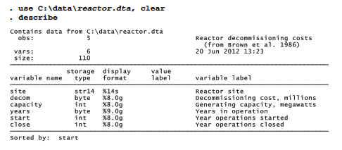
Dataset reactor.dta contains information about the decommissioning costs of five nuclear power plants that were shut down over 1968-1982. This example has the pedagogical advantage that its small matrices could be written easily on blackboard or paper, if desired (e.g., Hamilton 1992a:340). In any event, it invites the question of how decommissioning costs might be related to reactor capacity and years of operation.
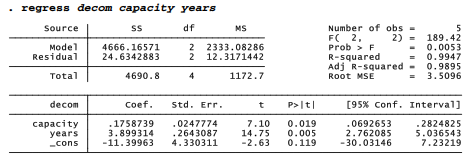
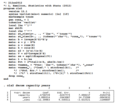
Performing OLS regression with Stata is very easy, of course. We find that decommissioning costs among these five reactors increased by about .176 million dollars ($175,874) with each megawatt of generating capacity, and by about 3.9 million dollars with each year of operation. The two predictors explain almost 99% of the variance in decommissioning costs (R2a = .9895).
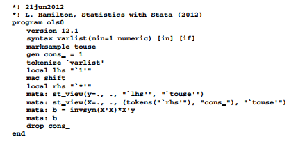
The ado-file below defines program ols0 using Mata commands. It simply calculates the vector of regression coefficients b. Mata commands start with mata: in this example. (Several other ways to use these commands interactively or in programs are described in the manuals.) The first two mata: commands define vector y and matrix X as “views” of the data in memory, specified by whatever left-hand-side (lhs) and right-hand-side (rhs) variables appeared in the ols0 command line. A constant, 1, forms the last column of matrix X. ols0 permits in or if qualifiers, or missing values. The estimating equation
b = (X’X) -1 X’y
is written in Mata as
mata: b = invsym(X’X)*X’y
The fourth mata: command displays the resulting contents of b.
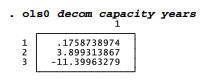
Applied to the reactor decommissioning data, ols0 obtains regression coefficients identical to those found earlier by regress
Using Mata versions of the standard equations, program olsl (next page) adds the calculation of standard errors, t statistics, and t test probabilities. Again, the calculations lead to the same results we saw earlier with regress. Commas in the final mata statement of olsl are operators, meaning “join the columns of the following matrices.”
*! 21jun2012
*! L. Hamilton, Statistics with Stata (2012) program ols1
version 12.1
syntax varlist(min=1 numeric) [in] [if]
marksample touse
gen cons_ = 1
tokenize ‘varlist’
local lhs “‘1′”
mac shift
local rhs “‘*'”
mata: st_view(y=., ., “‘lhs'”, “‘touse'”)
mata: st_view(X=., ., (tokens(“‘rhs'”), “cons_”), “‘touse'”)
mata: b = invsym(X’X)*X’y
mata: e = y – X*b
mata: n = rows(X)
mata: k = cols(X)
mata: s2 = (e’e)/(n-k)
mata: V = s2*invsym(X’X)
mata: se = sqrt(diagonal(V))
mata: (b, se, b:/se, 2*ttail(n-k, abs(b:/se)))
drop cons_
end

We could expand this program to store results, and post them in a nicely-formatted output table similar to that of regress. Program ols2 (next page) accomplishes something different, in order to demonstrate how Mata joins matrices together. It combines the numerical results seen above into a string matrix that also contains column headings and a list of independent-variable names. This happens through several additional mata commands. One defines row vector vnames_ containing a list of variable names. The commas in this expression join three sets of columns: (1) the word “Yvar:” followed by the left-hand-side variable’s name; (2) the names of all right- hand-side variables; and (3) the word “_cons”.
mata: vnames_ = “Yvar: ‘lhs'”, tokens(“‘rhs'”), “_cons”
The next long mata command uses within-line comment delimiters, /* and */, so that Mata reads past the end of two physical lines and sees this as all one command:
mata: vnames_’, (“Coef.” \ strofreal(b)), /*
*/ (“Std. Err.” \ strofreal(se)), /*
*/ (“t” \ strofreal(t)), (“P>|t|” \ strofreal(Prt))
The command displays a matrix in which the first column is the transpose of vnames_ (that is, a column of variable names). The column of variable names is joined, using a comma, to a second column vector created with the word “Coefs” as its first row; remaining rows are filled by the coefficients in b converted from real numbers to strings. The backslash operator “\” joins rows to a matrix, just as “,” joins columns. The real-to-string conversion of b values is necessary to make the matrix types compatible. Similar operations in ols2 form labeled columns of standard errors, t statistics, and probabilities.
These Mata exercises, like other examples in this chapter, give only a glimpse of Stata programming. The Stata Journal publishes more inspired applications, and each update of Stata involves new or improved ado-files. Online NetCourses provide a guided route to fluency in writing your own programs.
Source: Hamilton Lawrence C. (2012), Statistics with STATA: Version 12, Cengage Learning; 8th edition.
23 Sep 2022
26 Sep 2022
28 Sep 2022
3 Oct 2022
1 Oct 2022
23 Sep 2022