How to Use Plugins to Create a Model Instead of Drawing a Model in AMOS

If you do not want to use the graphical interface to conceptualize your model, AMOS does have an option where you can use a syntax option to run your analysis. Numerous SEM pro- grams in the past were solely syntax based, and if you feel more comfortable typing in the rela- tionships than using the graphical interface, AMOS provides you with that option.This option is usually slower, but it does give you a nice documentation of the model and relationships when the coding is complete. As well, learning to code the data is a skill that is transferable to other statistical packages. Lastly, if you want to collaborate with other authors who only know how to use syntax, you can now speak a common language in the collaboration process.AMOS uses a form of Visual Basic that allows you to specify a model in text form.

AMOS uses “pd” functions that will represent an object in the graphics window. Here is a list of the five most prominent functions.

With each one of these functions, you need to make sure all data file names of variables and names of unobservable variables you created have a quotation mark at the beginning and ending of the name. AMOS will not know what variable you are trying to access without those quotation marks. A single program line in the coding format will equate to a single object added in the model or functions needed in the model.

Let’s look at how we could use the Plugins function via syntax to run a confirmatory fac- tor analysis. After this example, I will show you how to code a full structural model.The CFA example will be the same one we used in Chapter 4. We will start with a simple three con- struct factor analysis of the constructs of Adaptive Behavior, Customer Delight, and Positive Word of Mouth. We are going to model the observables for each construct along with all the error terms for each observable. To see what the model initially looked like in the graphics window, see Figure 10.49.

Figure 10.49 CFA Model From Chapter 4

There are two ways to code the data in AMOS. The first way is through the “program edi- tor” software in AMOS.This not located in the graphics window.The program editor is a sepa- rate program that is solely code based (it will not draw a model).The second option is located in the graphics window and is located in the Plugins option at the top.The Plugins option will allow you to specify the model in a coding format, and then AMOS creates the model in the graphics window. I find this second option a little easier because you can still use the Analysis Properties button in the graphics window to specify different analysis options. I will show you both methods for coding the data, but let’s first start with the “Plugins” option in the graphics window first.

Figure 10.50 Plugins Window in AMOS

We first need to go to the AMOS graphics window and then select the “Plugins” option at the top right and then select “Plugins”. A pop-up window will appear with the default plugins listed (see Figure 10.50).You can also hit ALT+F8, and it will take you directly to this pop-up window. When the pop-up window appears, hit the “Create” button. This will bring up a program editor window with some default code already in the window. The first three functions will be “Name”, which is the name you want to call this plugin; “Description”, which is a brief description that can be entered about the model or file; and “Mainsub”, which is the area where you will input the code that will tell AMOS what to turn into a graphic.

Figure 10.51 Plugins Window in AMOS

I am going to call this plugin “CFA Syntax”, and I am going to include a description of the file as “CFA analysis using Syntax function”.

Figure 10.52 Name and Description Included in Plugin

Under the “Mainsub” function, we are initially going to enter all the unobservables and observables in the model. I am going to initially input all the indicators of the unobservable constructs. Adaptive Behavior had five indicators, while Positive Word of Mouth and Cus- tomer Delight had three indictors each. To input these observables, we are going to use the “pd. Observed” function. For the first Adaptive Behavior indicator (adapt1), we are going to let AMOS know this is an observable in the model by coding it:

pd.Observed (“adapt1”)

Make sure you include the parenthesis and quotation marks in this line function. Next, we are going to include all the rest of the indicators. See Figure 10.53.

Figure 10.53 Observable Variables Coded in Plugin

Notice that I included a line space between the construct’s indicators; this just helps to keep the code orderly instead of a huge list of indicators.You want to make sure you can easily see if you are missing an indicator for a construct.

Underneath the observables, we can start to include the unobservables.The unobservables will use the following function:

Pd. Unobserved (“construct name”)

The first construct of Adaptive_Behavior is coded as: pd. Unobserved (“Adaptive_Behavior”). I will code the other unobservable constructs the same way.

The error terms in our model are also considered unobservables. Each indicator has an error term that needs to be coded as an unobservable. The “unobservable” error terms are coded the same way as the unobservable constructs.The first error term of “e1” is coded as:

pd.Unobserved (“e1”)

We will code all the other error terms the exact same way. Again, it is okay to have a blank line between your coding in order to organize your coding into areas.

Figure 10.54 Unobservable Variables Coded in Plugin

After telling AMOS what the unobservable and observable items are in the model, you can then add single headed or double headed arrow relationships in the model.You can also start to code any constraints that are in the model. Let’s start with adding the single headed arrow relationships in the CFA.We are going to use the “pd. Path” function next.When using the path function, you have to denote where the arrow is pointing to and where it is pointing from in the code.You also have to denote if the relationship has a constraint. Here is how the function is set up:

pd. Path (“object where the arrow is pointing to”, “object where the arrow is pointing from”, constraint)

In the Adaptive Behavior construct, let’s model the first indicator (adapt1). This indicator is also constrained to 1 because it is setting the metric for the construct. Here is how to code this relationship:

pd. Path (“adapt1”, “Adaptive_Behavior”, 1)

The unobserved Adaptive Behavior construct has a reflective path to its indicator of adapt1 and the path is constrained to 1. If we had no constraint in the path, then we would not include any value at the end of the line function. For instance, the next indicator to be coded for Adaptive Behavior would be: pd. Path (“adapt2”, “Adaptive_ Behavior”). You will need to code the relationship for each unobservable construct to its indicators. Make sure to code the constraint in each construct for the indicator that sets the metric.

After coding the paths from the unobservable construct to the indicators, you now need to code the error term relationships. The error terms are classified as unobservables, so they will be coded the same way as the unobservable constructs were just coded. One specific dif- ference is that all error terms have a constraint of 1 in its relationship.When you are drawing your model using the graphics interface, AMOS will put this constraint in by default; but in the program editor window, you will have to specifically tell AMOS to put a constraint in the relationships from the error term to the indictors.

Let’s now try to code the error term for the adapt1 indicator. The error number can be whatever number you choose, but to be consistent with the example from Chapter 4 where we drew the model in the graphics window, the error term is “e7”.To code this relationship, it would be:

pd.Path (“adapt1”, “e7”, 1)

We would then need to code all the error terms for each indicator, making sure that every indicator had a constraint of 1 added.

Figure 10.55 Coding the Relationships to Indicators and Error Terms

With a CFA, all unobservable constructs are considered independent constructs. Thus, all independent constructs need to be covaried.To do this, we will use the covariance function of “pd. Cov”. Here is an example of the covariance function:

pd. Cov (“Adaptive_Behavior, “Customer_Delight”)

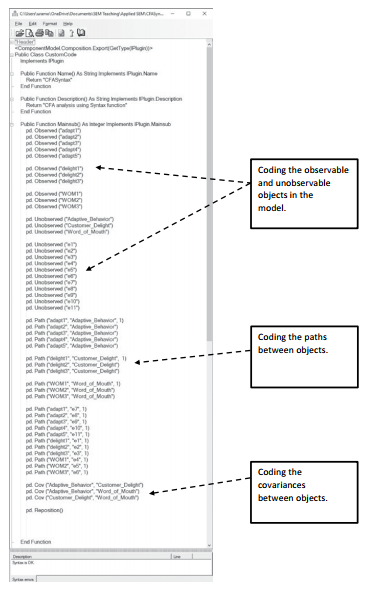
Figure 10.56 Total Code for the CFA Plugin

You will notice at the bottom of the Mainsub section I included a function that was listed as

pd. Reposition ()

This function will group the observable and error terms together with an unobservable con- struct when AMOS creates the model in the graphics window. If you don’t specify this func- tion, the model is going to have observables and unobservables just randomly placed on the graphics screen.

This is all the coding we need to enter into the Mainsub area. There is much more coding below this area, but it is fine to leave those blank at this point. Next, you need to check the syntax to make sure you do not have any errors. At the top of the screen are some icons.

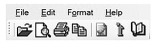
Figure 10.57 Icons on Plugin Coding Screen

The icon with the checkmark on the page is the check syntax function. Once you have clicked this, you should get a “Syntax is Ok” message in the description section under the cod- ing if no errors are present. If an error does occur, the error message will be displayed in the description section.

After checking your syntax, you need to save your coding.To run the coding in the AMOS graphics window, you need to save this file in the AMOS Plugins folder. If you do not save it in this folder, the graphics window will not be able to access and run the analysis.The location you need to save this file is typically:

C:\Users\username\Appdata\Local\AmosDevelopment\AMOS\26\Plugins

You can always hit the “Save As” button, and it should default into this location or the loca- tion that you specifically need to save the coding. Again, if it is not saved in the Plugins folder, AMOS can not run the analysis.

Once you save the file, you should see that Plugin is one of the default names when you click into the Plugin option on the graphics screen.You will also see at the bottom the descrip- tion of the Plugin.

Figure 10.58 CFA Syntax Listed in Plugin Window

To launch the Plugin, you need to create a new file in the AMOS graphics window and then read in the data file you want to use with the select data file icon . Next, you will go to the Plugins option and then select your file, which was named CFA Syntax in this example.

AMOS will conceptualize the model in the graphics window. Here is what the model looks like after running the Plugin:

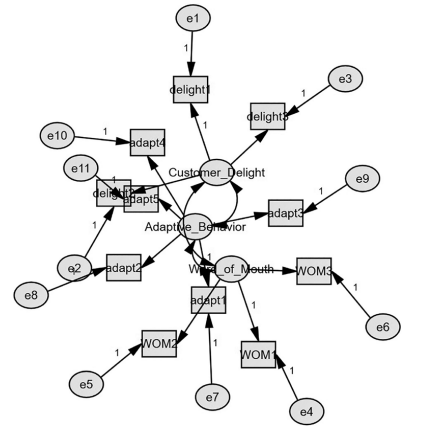
Figure 10.59 CFA Syntax Plugin Modeled in Graphics Window

I know that after looking at the model drawn by AMOS, many of you are thinking “Wow, this is a hot mess! I thought the reposition function we added was going to group the denoted objects around an unobservable construct”.You are correct, the reposition function helps AMOS organize the model; this is the best AMOS can do without you specifically noting where you want each construct based on a pixel location, which is a very laborious process. Figure 10.60 shows you what the model looks like when the reposition function is not included in the coding.

Figure 10.60 CFA Syntax Plugin with Reposition Code Removed

If you are using syntax in the Plugins function to draw the model in AMOS graphics, you probably do not really care what the model looks like; you are just concerned with the analy-sis. Once the model has been drawn, then you can use the calculate estimates button to run the analysis. The results of this analysis are the exact same as the test we performed in Chapter 4.

Using the syntax function with the Plugins function does have advantages and disadvan- tages. One of the disadvantages is you are going to see every model created listed in the Plugins function in the drop-down menu. I do not want to see every possible model I have created, because that could be a very long list. You can create the coding file and save it in another location and then simply copy it into the Plugins folder when you are ready to use it. By doing it this way, you see only the default plugins and then the file you just copied in. This is a work-around, but still a little bit of a hassle.

Another disadvantage is that the model that is created in the AMOS graphics window is hard to see and not very easy to interpret.You would almost need to go back into the coding to see the relationships or spend a lot of time fixing the model to make it graphically pleasing. The graphics window part is not that helpful with this function.

There are some advantages to using this function as well. While I do not prefer to code a whole model in this function, if you have a repetitive construct that you use continually, you can code the construct, its indicators, and error terms in the plugin for future use. For instance, if you consistently use an “Involvement” scale that was 13 items in the data set, you could code the unobservables and observables of the involvement construct and save it to the Plugins folder. When you were ready to include that construct in your model, you could use the plugin and save some time from creating a new 13-indicator construct every time. Addi- tionally, if a construct-to-construct relationship is consistently being modeled, this Plugins function will save you some effort instead of creating the constructs in the model every time. You do need to make sure to call the specific observables the same name across your data sets if you use the Plugins function for this, or AMOS will not be able to anlayze the data because of the different observable’s names listed in the data and in the model. The biggest advantage to coding the data this way is the flexibility it gives you in the analysis.You can code the unob- servables and observables in the model along with relationships but can still use the analysis icons to select options and text viewing in an easy manner compared to coding all the requests in the program editor. It is kind of like the best of both worlds. You can use syntax code to conceptualize the model and then use the icon functions to denote options in the analysis. For functions like two group analysis and invariance testing, this option is substantially easier than the alternative of coding every analysis option needed in the program editor software.

Before examining how to use the dedicated program editor software, I want to give you one more example of plugin coding for a full structural model. In our example, we just examined the measurement model, but this time let’s examine a full structural model where the meas- urement and the structural relationships are included.

I am going to call this plugin “StructuralTest”, and it will include a simple description of a “full structural model test of Adaptive Behavior, Customer Delight, and Positive Word of Mouth”. This model test will examine how Adaptive Behavior influences Customer Delight which influences Positive Word of Mouth.The initial coding of unobservables and observables will be exactly the same, but we are going to add error terms to the dependent variables and relationships between the constructs. We will also remove all the covariances between the constructs because now we only have one independent construct. See Figure 10.61 for the coding of the structural model test.

Figure 10.61 Plugin’s Code for a Full Structural Model

Source: Thakkar, J.J. (2020). “Procedural Steps in Structural Equation Modelling”. In: Structural Equation Modelling. Studies in Systems, Decision and Control, vol 285. Springer, Singapore.