Determining Research Sample Size

Determining the size of a sample really comes down to estimating the mini­mum size needed to obtain results with an acceptable degree of confidence. For samples destined for quantitative data processing this means determining the size that enables the study to attain the desired degree of precision or signi­ficance level; for qualitative research it is the size that confers an acceptable credibility level.

As a general rule, and all else being equal, the larger the sample, the greater the confidence in the results, whatever type of data processing is used. However, large samples pose problems of practicality, particularly in terms of cost and scheduling. Beyond a certain size, they can also pose problems in terms of relia­bility, for when a sample is very large, the researcher is often required to farm out data collection. This can increase the number of collection, recording and encoding errors – and may require the instigation of sometimes elaborate veri­fication procedures. Large samples can also turn out to be unnecessarily costly. For example, a small sample is sometimes sufficient to obtain a significant result when the effect of a variable in an experimental design has to be tested.

Determining the appropriate sample size before collecting data is essential in order to avoid the ex post realization that a sample is too small. Calculating the sample size required involves evaluating the feasibility of the research’s objectives, and, in certain cases, can lead to modifying the research design.

1. Samples Intended for Quantitative Processing

The size required for a sample intended for quantitative data processing depends on the statistical method used. Our intention here is not to provide formulae, but simply to present the factors common to most methods that influ­ence the sample size needed. There are many such factors: the significance level, the desired level of precision, the variance of the studied phenomenon in the population, the sampling technique chosen, the size of the effect being studied, the desired power of the test and the number of parameters to estimate. Which ones need to be taken into consideration depend on the purposes of the study. Nevertheless, two main categories of objectives can be distinguished: describing a population and testing a hypothesis.

1.1. Descriptive research

The principal evaluation criterion for descriptive research is usually precision. Precision depends on several factors: the desired significance level, the popu­lation variance and the sampling technique used. To illustrate the incidence of these factors on sample size, we will consider a very familiar statistic: the mean.

Example: Calculating sample size to estimate a mean

In the case of a simple random sample of more than 30 elements selected with or without replacement, but with a sampling ratio smaller than 10 per cent, to reach the desired level of precision, the minimum sample size is

where l is the level of precision, s is the population’s standard deviation, ■ the sample size, and z the value of the normal distribution for the significance level.

Population variance and sample size The larger the variance s², the larger the sample needs to be. Very often, however, the variance of the population is unknown. In that case, it must be estimated in order to calculate the size of the sample. There are several possible ways of doing this. The first is to use results of earlier studies that give suggested variance estimates. Another solution is to perform a pilot study on a small sample. The variance calculated for this sam­ple will provide an estimate for the population variance. A third solution is based on the assumption that the variable being studied follows a normal dis­tribution, which is unlikely for many organizational phenomena. Under this assumption, the standard deviation is approximately one-sixth of the distribu­tion range (maximum value minus minimum value). Finally, when a scale is used to measure the variable, one can refer to the guidelines below.

Significance level and sample size Significance level (a) refers to the possibil­ity of rejecting the null hypothesis when it should not have been rejected. By convention, in management research accepted levels are generally from 1 per cent to 5 per cent, or as much as 10 per cent – depending on the type of research. The 1 per cent level is standard for laboratory experiments; for data obtained through fieldwork, 10 per cent could be acceptable. If the significance level is above 10 per cent, results are not considered valid in statistical terms. The desired significance level (a) has a direct influence on sample size: the lower the accept­able percentage of error, the larger the sample needs to be.

Precision level and sample size The precision level (l) of an estimate is given by the range of the confidence interval. The more precise the results need to be, the larger the sample must be. Precision is costly. To increase it twofold, sample size must be increased fourfold.

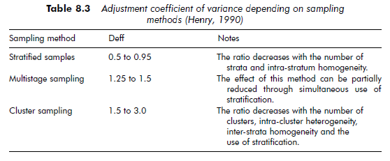
Sampling method and sample size The sampling method used affects samp­ling variability. Every sampling method involves a specific way of calculating the sample mean and standard deviation (for example, see Kalton, 1983). Consequently, sample size cannot always be calculated with the simple formula used in the example on page 158, which is valid for a simple random sample only. However, no matter which sampling method is chosen, it is possible to estimate sample size without having to resort to complex formulae. Approxi­mations can be used. Henry (1990), for example, presents several ‘design effect’ – or deff – adjustment coefficients (see Table 8.3).

By applying these coefficients, sample size can be estimated with a simple calculation derived from the basic formula. The variance is multiplied by the coefficient corresponding to the method used (s’² = s². deff).

Returning to the formula we used above, with a simple random sample the size is:

 

With a multistage sample, the maximum deff coefficient is 1.5, so the size is:

1.2. Hypothesis testing

Other criteria must also be taken into account in the case of samples that will be used to test hypotheses (the most common use of samples in research work). These include effect size, the power of the statistical test and the number of parameters to estimate. These criteria help us to ascertain the significance of the results.

Effect size and sample size Effect size describes the magnitude or the strength of the association between two variables. Indices measuring effect size depend on the statistics used.

If we take, for example, the test of difference between means, and we assume that the standard deviation is the same for both samples, effect size is given by the ratio d:

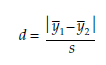
For example, if the average y₁of the studied variable in the first sample is 33, the mean y₂ of the second is 28, and the standard deviation s is 10 for each sample, the effect size will be 50 per cent (d = (33 – 28)/10 = 0.5).

Effect sizes are generally classified into three categories: small, medium and large. A 20 per cent effect is considered small, a 50 per cent effect medium and an 80 per cent effect large (Cohen, 1988). In terms of proportion of variance, accounted for by an independent variable, these three categories correspond to the values 1 per cent, 6 per cent and 14 per cent.

The smaller the effect the larger the sample size must be if it is to be statistically significant. For example, in a test of difference between means, with two identically sized samples, if the required size of each sample is 20 for a large effect, it will be 50 for a medium one and 310 for a small effect, all else being equal.

Estimating effect size is not easy. As for variance, we can use estimates from earlier research or do a pilot study with a small sample. If no estimate exists, we can also use the minimum effect size that we wish to obtain. For example, if an effect of less than 1 per cent is deemed worthless, then sample size must be calculated with an effect size of 1 per cent.

For management research effect sizes are usually small, as in all the social sciences. When analyzing 102 studies about personality, Sarason et al. (1975) noticed that the median percentage of variance accounted for by an indepen­dent variable ranged from 1 per cent to 4.5 per cent depending on the nature of the variable (demographics, personality or situation).

The power of the test and sample size The power of the test could be interpreted as the likelihood of being able to identify the studied effect. When it is low, we cannot determine whether there is no relation between the vari­ables in the population, or whether a relation exists but was not significant because the research was not sufficiently sensitive to it.

The power of the test is expressed with the coefficient (1 – β) (see Chapter 11, Comparison Tests).

For example, a power of 25 per cent (1 -β = 0.25) means that there is only a 25 per cent chance of correctly rejecting the null hypothesis H₀: that is, there is a 75 per cent chance that no conclusion will be drawn.

The power of the test is rarely mentioned when presenting results, and is not often considered in management sciences (Mazen et al., 1987). Most research presents significant effects only, i.e. for which the null hypothesis H₀ has been able to be rejected. In this case, the decision error is the Type I error a. So it is not surprising to see that Type II error P is not mentioned, since it means accept­ing H₀ when it is not true.

Cohen (1988) defined standards for β error of 20 per cent and 10 per cent. They are not as strict as those generally accepted for significance level α (5 per cent and 1 per cent). The power of the test depends on the significance level. The relationship between a and β is complex, but, all else being equal, the lower a is, the higher β becomes. Still, it is not advisable to reduce Type II error by increasing Type I error, because of the weight of convention concerning α error. There are other means of improving power. For a given a error, the power of the test increases when sample size increases and variance decreases. If, despite everything, the power of the test is still not acceptable, it may be reasonable to give up on the test in question.

In research comparing two samples, increasing the size of one of them (the control sample) is another way of increasing the power of the test.

When replicating research that did not lead to a rejection of the null hypo­thesis, Sawyer and Ball (1981) suggest estimating the power of the tests that were carried out – this can be calculated through the results of the research. If
the power appears low, it should be increased in order to raise the chance of obtaining significant results. Cook and Campbell (1979) also advise presenting the power of the test in the results when the major research conclusion is that one variable does not lead to another.

Sample size and number of parameters to estimate Sample size also depends on the number of parameters to be estimated, that is, the number of variables and interaction effects which are to be studied. For any statistical method, the larger the number of parameters that are to be estimated, the larger the sample should be.

When more elaborate statistical methods are used, determining the sample size required in order to achieve the desired significance becomes extremely complex. For means and proportions, simple calculation formulae exist and can be found in any statistics handbook (for example, see Thompson, 1992). On the other hand, for more complicated methods, for example, regression, there are no simple, comprehensive formulae. Researchers often imitate earlier studies for this reason. For most methods, however, calculation formulae or tables exist which enable researchers to estimate sample size for one or more criteria. Rules of thumb often exist as well. These are not, of course, as precise as a formula or a table, but they may be used to avoid major mistakes in estimating sample size.

1.3. Usable sample size

The indications presented above for determining sample size concern only the usable sample size – that is, the number of elements retained for statistical analysis. In a random sampling technique, each element selected should be part of the usable sample. If that is not the case, as we mentioned in the first section, then there is bias. It is unusual in management research, though, to obtain all the desired information from each of the randomly selected elements. The rea­sons for this are many, but they can be classified into four main categories: impossibility of contacting a respondent, refusal to cooperate, ineligibility (that
is, the selected element turns out not to belong to the target population) and responses that are unusable (for example, due to incompleteness). The response rate can vary tremendously, depending on a great number of factors related to the data collection methods used (sampling method, questionnaire adminis­tration technique, method used to contact respondents, etc.), the nature of the information requested or the amount of time required to supply it. The response rate can often be very low, particularly when data is being gathered through self-administered questionnaires. Certain organizational characteristics can also affect the response rate. The respondent’s capacity and motivation can similarly depend on organizational factors (Tomaskovic-Devey et al., 1994). For example, when a questionnaire is addressed to a subsidiary, but decision-making is cen­tralized at the parent company, response probability is lower.

The likely response rate must be taken into account when determining the size of the sample to be contacted. Researchers commonly turn to others who have collected similar data in the same domain when estimating this response rate.

Samples used in longitudinal studies raise an additional problem: subject attrition – that is, the disappearance of certain elements (also referred to as sample mortality). In this type of study, data is gathered several times from the same sample. It is not unusual for elements to disappear before the data collec­tion process is complete. For example, when studying corporations, some may go bankrupt, others may choose to cease cooperating because of a change in management. In researching longitudinal studies published in journals of indus­trial psychology and organizational behavior, Goodman and Blum (1996) found attrition rates varied from 0 to 88 per cent with a median rate of 27 per cent. In general, the longer the overall data-collection period, the higher the attrition rate. Researchers should always take the attrition rate into account when calcu­lating the number of respondents to include in the initial sample.

1.4. Trading-off sample size and research design

As discussed above, sample size depends on the variance of the variable under study. The more heterogeneous the elements of the sample are, the higher the variance and the larger the sample must be. But it is not always feasible, nor even necessarily desirable, to use a very large sample. One possible answer to this problem is to reduce variance by selecting homogenous elements from a subset of the population. This makes it possible to obtain significant results at lower cost. The drawback to this solution is that it entails a decrease in external validity. This limitation is not, however, necessarily a problem. Indeed, for many studies, external validity is secondary, as researchers are more concerned with establishing the internal validity of results before attempting to generalize from them.

When testing hypotheses, researchers can use several small homogenous samples instead of a single, large heterogeneous sample (Cook and Campbell, 1979). In this case, the approach follows a logic of replication. The researcher tests the hypothesis on one small, homogenous sample, then repeats the same analysis on other small samples, each sample presenting different characteristics. To obtain the desired external validity, at least one dimension, such as popula­tion or place, must vary from one sample to another. This process leads to a high external validity – although this is not a result of generalizing to a target population through statistical inference, but rather of applying the principles of analytic generalization across various populations. The smaller samples can be assembled without applying the rigorous sampling methods required for large, representative samples (Cook and Campbell, 1979). This process also offers the advantage of reducing risks for the researcher, in terms of time and cost. By limi­ting the initial study to a small, homogenous sample, the process is simpler in its application. If the research does not produce significant results, the test can be performed on a new sample with a new design to improve its efficiency. If that is not an option, the research may be abandoned, and will have wasted less labor and expense than a test on a large, heterogeneous sample.

A similar process using several small samples is also an option for researchers studying several relations. In this case the researcher can test one or two variables on smaller samples, instead of testing all of them on a single large sample. The drawback of this solution, however, is that it does not allow for testing the inter­action effect among all the variables.

2. Samples Intended for Qualitative Analysis

In qualitative research, single-case studies are generally differentiated from multiple-case studies. In fact, single case studies are one of the particularities of qualitative research. Like quantitative hypothesis testing, sample size for quali­tative analysis also depends on the desired objective.

2.1. Single case studies

The status of single-case studies is the object of some controversy. Some writers consider the knowledge acquired from single case studies to be idiosyncratic, and argue that it cannot be generalized to a larger or different population. Others dispute this: for example, Pondy and Mitroff (1979) believe it to be per­fectly reasonable to build theory from a single case, and that the single-case study can be a valid source for scientific generalization across organizations. According to Yin (1990), a single-case study can be assimilated to an experi­ment, and the reasons for studying a single case are the same as those that motivate an experiment. Yin argues that single case studies are primarily justi­fied in three situations. The first is when testing an existing theory, whether the goal is to confirm, challenge or extend it. For example, Ross and Straw (1993) tested an existing prototype of escalation of commitment by studying a single case, the Shoreham nuclear-power plant. Single cases can also be used when they have unique or extreme characteristics. The singularity of the case is then the direct outcome of the rarity of the phenomenon being studied. This was the case, for example, when Vaughan (1990) studied the Challenger shuttle disas­ter. And finally, the single-case study is also pertinent if it can reveal a pheno­menon which is not rare but which had until now been inaccessible to the scientific community. Yin points to Whyte’s (1944) research in the Italian com­munity in poor areas of Boston as a famous example of this situation.

2.2. Multiple cases

Like quantitative analysis, the confidence accorded to the results of qualitative research tends to increase with sample size. The drawback is a parallel increase in the time and cost of collecting data. Consequently, the question of sample size is similar to quantitative samples – the goal is to determine the minimum size that will enable a satisfactory level of confidence in the results. There are essentially two different principles for defining the size of a sample: replica­tion and saturation. While these two principles are generally presented for determining the number of cases to study, they can also be applied to respondent samples.

Replication The replication logic in qualitative research is analogous to that of multiple experiments, with each case study corresponding to one experiment (Yin, 1990). The number of cases required for research depends on two criteria, similar to those existing for quantitative samples intended for hypothesis test­ing. They are the desired degree of certainty and the magnitude of the observed differences.

There are two criteria for selecting cases. Each case is selected either because similar results are expected (literal replication) or because it will most likely lead to different results for predictable reasons (theoretical replication). The number of cases of literal replication required depends on the scale of the observed differences and the desired degree of certainty. According to Yin (1990), two or three cases are enough when the rival theories are glaringly different or the issue at hand does not demand a high degree of certainty. In other circumstances, when the differences are subtle or the required degree of certainty is higher, at least five or six literal replications would be required.

The number of cases of theoretical replication depends on the number of conditions expected to affect the phenomenon being studied. As the number of conditions increases, so does the potential number of theoretical replications. To compare it to experimentation, these conditions of theoretical replication in multiple case studies fulfill the same purpose as the different conditions of observation in experimental designs. They increase the internal validity of the research.

The saturation principle Unlike Yin (1990), Glaser and Strauss (1967) do not supply an indication for the number of observation units a sample should contain. According to these authors, the adequate sample size is determined by theoretical saturation. Theoretical saturation is reached when no more information will enable the theory to be enriched. Consequently, it is impossible to know in advance what the required number of observation units will be.

This principle can be difficult to apply, as one never knows with absolute certainty if any more information that could enrich the theory exists. It is up to the researcher therefore, to judge when the saturation stage has been reached. Data collection usually ends when the units of observation analyzed fail to supply any new elements. This principle is based on the law of diminishing returns – the idea that each additional unit of information will supply slightly less new information than the preceding one, until the new information dwindles to nothing.

Above and beyond these two essential principles, whose goal is raising internal validity, it is also possible to increase the number of cases in order to improve external validity. These new cases will then be selected in such a way as to vary the context of observation (for example, geographical location, industrial sector, etc.). Researchers can also take the standard criteria of credibility for the community to which they belong into account when determining the number of elements to include in a sample intended for qualitative processing.

Source: Thietart Raymond-Alain et al. (2001), Doing Management Research: A Comprehensive Guide, SAGE Publications Ltd; 1 edition.