Selecting Research Sample Elements

1. Sampling Methods

External validity can be achieved by employing one of two types of inference: statistical or theoretical. Statistical inference uses mathematical properties to generalize from results obtained from a sample to the population from which it was taken. Theoretical inference (or analytical generalization) is another form of generalization, but one that is not based on mathematical statistics. Rather than aiming to generalize from statistical results to a population, theoretical inference aims to generalize across populations on the basis of logical reasoning.

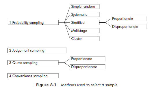
The different sample selection methods can be grouped into four categories (see Figure 8.1). These categories do not employ the same modes of inference. The first category is made up of probability sampling methods, in which each element of a population has a known probability, not equal to zero, of being selected into the sample. These are the only methods that allow the use of statistical inference.

Unlike probability sampling, in which researcher subjectivity is to be elimi­nated as far as possible, the second category is composed of methods based on personal judgement. Elements are selected according to precise criteria, estab­lished by the researcher. The results obtained from a judgement sample lend themselves to an analytical type of generalization.

The third category corresponds to the quota method. Not being a probability sampling method, quota sampling does not, strictly speaking, allow for statisti­cal inference, however, in certain conditions which will be described later, quota sampling can be similar to probability sampling, and statistical inference can then be applied.

Convenience sampling methods make up the fourth group. This term desig­nates samples selected strictly in terms of the opportunities available to the researcher, without applying any particular criteria of choice. This selection method does not allow for statistical inference. Nor does it guarantee the possi­bility of theoretical inference, although an ex post analysis of the composition of the sample may sometimes allow it. For this reason, convenience sampling is generally used in exploratory phases only, the purpose being to prepare for the next step, rather than to draw conclusions. In this context a convenience sample can be sufficient, and it does present the advantage of facilitating and accelera­ting the process of data collection.

The choice of methods is often restricted by economic reasons and reasons of feasibility. Nonetheless, the final decision in favor of a particular method must always be based on the objectives of the study.

1.1. Probability sampling

Probability sampling involves selecting elements randomly – following a random procedure. This means that the selection of any one element is independent of the selection of the other elements. When trying to estimate the value of a certain parameter or indicator, probability samples allow researchers to calculate how precise their estimations are. This possibility is one advantage of probability sampling over other selection methods.

Two elements distinguish among different types of probability sampling methods:

• The characteristics of the sampling frame: whether the population is com­prehensive or not and whether the frame includes specific information for each population element.
• The degree of precision of the results for a given sample size.

Simple random sampling Simple random sampling is the most basic selection method. Each element of the population has the same probability of being selected into the sample – this is referred to as equal probability selection. The elements of the sampling frame are numbered serially from 1 to N, and a table of random numbers is used to select them.

The main disadvantage of simple random sampling is that a comprehensive, numbered list of the population is required. This method also tends to select geographically diverse elements, which can make data collection extremely costly.

Systematic sampling Systematic sampling is closely related to simple random sampling. Its main advantage is that it does not require a numbered list of the population elements. A systematic selection process selects the first element randomly from the sampling frame, then selects the following elements at con­stant intervals. The selection interval is inversely proportional to the sampling ratio of sample size n divided by population size N. For example, if the samp­ling ratio is 1/100, one element will be selected in the list every 100 elements. Nevertheless, it is important to ensure that the selection interval does not corres­pond to an external reality that could bias the outcome. For example, if the sampling frame supplies monthly data in chronological order and the selection interval is a multiple of 12, all the data collected will refer to the same month of the year.

In practice, this procedure is not always followed strictly. Instead of setting a selection interval in terms of the number of elements, a simple rule is often established to approach this interval. For example, if the sampling frame is a professional directory, and the selection interval corresponds to approximately three pages in the directory, an element will be selected every three pages: the fifth element on the page – for instance – if the first, randomly selected, element was in that position.

Stratified sampling In stratified sampling, the population is initially segmen­ted on the basis of one or more pre-established criteria. The method is based on the hypothesis that there is a correlation between the phenomenon under observation and the criteria chosen for segmenting the population. The aim is to create strata that are as homogenous as possible in terms of the variable in question. The precision of the estimates is greatest when the elements are homo­genous within each stratum and heterogeneous from one stratum to the other. Consequently, in order to choose useful segmentation criteria the researcher must have a reasonably good prior knowledge of both the population and the phenomenon under study. This can be achieved by, for example, examining the results of earlier research.

Sample elements will then be selected randomly within each stratum, according to the sampling ratio, which may or may not be proportional to the relative number of elements in each stratum. When sample size is identical, using a higher sampling ratio for strata with higher variance – to the detriment of the more homogenous strata – will reduce the standard deviation for the whole sample, thereby making the results more precise. A higher sampling ratio might also be used for a subset of the population that requires closer study.

Multistage sampling Multistage sampling makes repeated selections at dif­ferent levels. The first stage corresponds to the selection of elements called pri­mary units. At the second stage, subsets, called secondary units, are randomly selected from within each primary unit, and the procedure is repeated until the final stage. Elements selected at the final stage correspond to the units of analysis. One significant advantage of multistage sampling is that it does not require a list of all of the population elements. Also, when stages are defined using geo­graphical criteria, the proximity of the selected elements will, in comparison with simple random sampling, reduce the costs of data collection. The down­side of this method is that the estimates are less precise.

In multistage sampling it is entirely possible to choose primary units accord­ing to external criteria – in particular, to reduce data collection costs. This prac­tice does not transgress the rules of sampling. In fact, the only thing that matters is the equal probability selection of the elements in the final stage. The sampling ratio for the subsequent stages should however be lower, to compensate for the initial choice of primary unit.

Cluster sampling Cluster sampling is a particular type of two-stage sampling. The elements are not selected one by one, but by subsets known as clusters, each element of the population belonging to one and only one cluster. At the first stage, clusters are selected randomly. At the second, all elements of the selected clusters are included in the sample.

This method is not very demanding in terms of the sampling frame: a list of clusters is all that is required. Another important advantage is the reduction in data collection costs if the clusters are defined by a geographic criterion. The downside is that estimates are less precise. The efficiency of cluster sampling depends on the qualities of the clusters: the smaller and more evenly sized they are, and the more heterogeneous in terms of the studied phenomenon, the more efficient the sample will be.

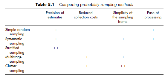
We should make it clear that these different sampling methods are not necessarily mutually exclusive. For instance, depending on the purposes of the study, multistage sampling might be combined with stratified sampling, the primary units being selected at random and the elements of the sample being selected into the primary units by the stratification method. One can also, for example, stratify a population, and then select clusters of elements within each stratum. This type of combination can raise the precision level of the estimations, while at the same time taking practical constraints into account (whether or not a comprehensive sampling frame exists, the available budget, etc.). Table 8.1 presents the advantages and disadvantages of each of these probability sampling methods.

1.2. Judgement sampling

The subjectivity of judgement sampling differentiates it from probability samp­ling, whose very purpose is to eliminate subjectivity. In management research, judgement samples, whether intended for qualitative or quantitative process­ing, are much more common than probability samples.

Unlike probability sampling, neither a specific procedure nor a sampling frame is needed to put together a judgement sample – as pre-existing sampling frames for organizational phenomena are rare, this is a definite advantage.

Even if it were theoretically possible to create one, the difficulty and the cost involved would often rule it out, although in some cases the snowball tech­nique can provide a solution (Henry, 1990). In addition, probability sampling is not always necessary, as research is often aimed more at establishing or testing a proposition than at generalizing results to a given population. For small samples, judgement sampling gives results that are just as good as those obtained from probability sampling, since the variability of the estimates for a small random sample is so high that it creates a bias equally great or greater than that result­ing from subjective judgement (Kalton, 1983). Furthermore, a sensitive research subject or an elaborate data collection system can bring about such elevated refusal rates that probability sampling does not make sense. Judgement sampling also allows sample elements to be selected extremely precisely, making it easier to guarantee respect for criteria such as homogeneity, which is required by certain research designs.

Judgement sampling does follow certain theoretical criteria, and to carry it out properly, the researcher must have a good working knowledge of the popu­lation being studied. The most common criterion is how ‘typical’, or conversely, ‘atypical’, the element is. Typical elements are those the researcher considers to be particularly ‘normal’ or ‘usual’ (Henry, 1990) in the population. A second criteria is the relative similarity or dissimilarity of the elements selected.

For both qualitative and quantitative research, selection criteria are guided by the desire to create either a homogenous or a heterogeneous sample. A homogenous sample will make it easier to highlight relationships and build theories. To put together such a sample, similar elements must be selected and atypical ones excluded. When research presenting strong internal validity has enabled a theory to be established, the results may be able to be generalized to a larger or a different population. In order to do this, dissimilar elements must be selected. For example, to increase the scope of a theory, Glaser and Strauss recommend varying the research field in terms of organizations, regions, and/or nations (Glaser and Strauss, 1967).

In experiments aimed at testing a relationship when it is difficult to select ran­dom samples large enough to provide significant external validity, one solution is to use samples composed of deliberately dissimilar elements (Cook and Campbell, 1979). The inference principle is as follows: as heterogeneity exercises a negative influence on the significance of the effect, if the relation appears significant despite this drawback, then the results can be generalized further.

1.3. Quota sampling

Quota sampling is a non-random sampling method that allows us to obtain a relatively representative sample of a population. There are a number of reasons for choosing quota sampling, for example, when the sampling frame is not available or is not detailed enough, or because of economical considerations.

As in stratified sampling, the population is segmented in terms of predefined criteria, in such a way that each member of the population belongs to one and only one segment. Each segment has a corresponding quota, which indicates the number of responses to be obtained. The difference between these two methods is found in the means of selecting sample elements, which in the quota method is not random. Two different types of procedures can be used.

The first type of procedure consists of filling the quotas as opportunities present themselves. The risk in this instance is that the sample might contain selection biases, since the first elements encountered may present a particular profile depending, for example, on the interviewer’s location, the sampling frame or other reasons.

The second type of procedure is called pseudo-random. For this a list of popu­lation elements (for example, a professional directory) is required, although, unlike stratified sampling, segmentation criteria are not needed for this list. The selection procedure consists of selecting the first element of the list at random, then going through the list systematically until the desired number of answers is reached. Even though this method does not scrupulously respect the rules of random sampling (the researcher does not know in advance the probability an element has of belonging to the sample), it does reduce potential selection bias by limiting subjectivity. Empirical studies have shown that the results are not significantly different from those obtained using probability sampling (Sudman, 1976).

2. Matched Samples

Experimental designs often use matched samples. Matched samples present similar characteristics in terms of certain relevant criteria. They are used to ascertain that the measured effect is a result of the variable or variables studied and not from differences in sample composition.

There are two principal methods of matching samples. The most common is randomization, which divides the initial sample into a certain number of groups (equal to the number of different observation conditions) and then ran­domly allocates the sample elements into these groups. Systematic sampling is often used to do this. For example, if the researcher wants to have two groups of individuals, the first available person will be assigned to the first group, the second to the second, the third to the first, etc. When the elements are hetero­geneous, this randomization technique cannot totally guarantee that the groups will be similar, because of the random assignment of the elements.

The second method consists of controlling sample structure beforehand. The population is stratified on the basis of criteria likely to affect the observed vari­able. Samples are then assembled so as to obtain identical structures. If the samples are large enough, this method has the advantage of allowing data processing to be carried out within each stratum, to show up possible strata differences.

According to Cook and Campbell (1979), matching elements before randomi­zation is the best way of reducing error that can result from differences in sam­ple composition. The researcher performs a pre-test on the initial sample, to measure the observed variable for each sample element. Elements are then classified from highest to lowest, or vice versa, in terms of this variable, and the sample is divided into as many equally sized parts as there are experimental conditions. For example, if there are four experimental conditions, the four elements with the highest score constitute the first part, the next four the second, etc. The elements in each part are then randomly assigned to experimental con­ditions. The four elements of the first part would be randomly assigned to the four experimental conditions, as would the four elements of the second part, and so on.

3. Sample Biases

Sample biases can affect both the internal and the external validity of a study. There are three categories of biases: sampling variability, sampling bias and non-sampling bias (although sampling variability and estimator’s bias affect probability samples only). The sum of these three biases is called the total error of the study (see Figure 8.2).

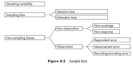
Sampling variability refers to differences that can be observed by comparing samples. Although one starts with the same population, samples will be com­posed of different elements. These differences will reappear in the results, which can, therefore, vary from one sample to another. Sampling variability decreases when sample size increases.

Sampling bias is related to the process of selecting sample elements or to the use of a biased estimator. In the case of a random sampling method, selection bias can crop up every time random selection conditions are not respected. Nevertheless, selection bias is much more common in non-random sampling, because it is impossible, by definition, for these methods to control the proba­bility that an element is selected into the sample. For example, quota sampling can lead to significant selection bias insofar as the respondents are, rather sub­jectively, selected by the investigator. Other sampling biases are related to the estimator selected. An estimator is a statistical tool that enables us to obtain, thanks to the data gathered from a sample, an estimate for an unknown para­meter, for example, variance. The mathematical construction of certain esti­mators presents the ‘proper’ properties, which establish the ‘proper’ estimates directly. When this is not the case, we say the estimator is biased.

Biases that are not related to sampling can be of different types, usually divided into two categories: non-observation biases and observation biases. The first can arise either from problems in identifying the study population, which we call coverage bias, or from lack of response. They can affect samples inten­ded for qualitative or quantitative processing. Observation biases, on the other hand, are associated with respondent error, or data-measurement, -recording or -encoding errors. Since observation biases do not stem from the constitution of the sample per se, in the following discussion we will consider non-observation- related biases only.

3.1. Non-coverage bias

A sample presents non-coverage bias when the study population does not corres­pond to the intended population, which the researcher wishes to generalize the results to. The intended population can encompass individuals, organizations, places or phenomena. It is often defined generically: researchers might say they are studying ‘small businesses’ or ‘crisis management’, for example. But researchers must take care to establish criteria that enable the population to be precisely identified. The set defined by the operationalization criteria will then constitute the study population. Two types of error can lead to a less than perfect correspondence between the intended population and the population under study: population-definition errors and listing errors.

Errors in defining the study population are one major source of bias. Inappropriately defined or insufficiently precise operationalization criteria can lead researchers to define the study population too broadly, or conversely, too narrowly. This type of error, for example, can result in different companies being selected for the same intended population. Not all of the sets defined in this way are necessarily pertinent in terms of the question being studied and the purpose of the research. This type of bias can occur in any type of sampling.

Example: Sources of error in defining the population

In a study of strategic choice in small businesses, the set ‘small businesses’ corres­ponds to the intended population. Nevertheless, it is important to establish criteria for defining an organization as a ‘small business’. Sales figures or the number of employees are two possible operationalization of the qualifier ‘small’. Similarly, ‘businesses’ could be defined in broad terms – as all organizations belonging to the commercial sector – or more restrictively – in terms of their legal status, including only incorporated organizations, and excluding non-profit and economic-interest groups. Choosing an overly strict operationalization of the definition, and including incorporated companies only, for example, will result in a sample that is not truly representative of the small business set. Partnerships, for example, would be exclu­ded, which could create a bias.

Listing errors are a potential cause of bias in the case of probability samples, for which the study population has been materialized as a sampling frame. They often result from recording errors or, even more commonly, from the insta­bility of the population being observed. For example, a professional directory published in 2000, used in the course of the following year will include com­panies that no longer exist and, conversely, will not include those which have been created since the directory was published. For practical reasons, it is not always possible to be rid of these errors. And yet, the validity of a study depends on the quality of the sampling frame. Researchers should therefore make sure that all the elements in the intended population are on the list, and that all the elements that do not belong to the population are excluded from it. The measures used to increase the reliability of the sampling frame can sometimes be ambiva­lent. For example, cross-referencing several lists generally helps to reduce the number of missing elements, but it can also lead to including the same element more than once, or to including elements that do not belong to the intended population. In the first case, the conditions of equal probability for each element are no longer maintained. In the second, bias appears which is comparable to the one presented above for definition error. Researchers can reduce these different types of errors before the sample is selected by scrupulously checking the sampling frame.

3.2. Non-response bias

Non-response bias can have two sources: the refusal of elements to participate in the study, or the impossibility of contacting a selected element or elements. If non-responses are not distributed randomly, the results can be biased. This is the case when non-response is connected to characteristics related to the study. For example, for research studying the effect of incentive programs on manage­rial behavior, non-response may correlate to a certain type of behavior (for example, interventionist) or with certain categories of incentive (for example, stock-option programs).

The higher the non-response rate, the greater the bias may be and the more likely it is to affect the validity of the research. The researcher should therefore try to avoid non-response. Several inducement techniques can be used for this purpose, generally dealing with methods to use when contacting and following up respondents, or with maintaining contact (this subject is dealt with in greater depth in Chapter 9). While these efforts may reduce the non-response rate, they rarely result in the researcher obtaining responses for the entire set of selected elements.

Different techniques can be applied to analyze non-response and, in certain circumstances, correct any possible bias of probability sampling results. These are presented at the end of this chapter, in the section on post sampling.

Because of non-coverage and non-response biases, the observed population hardly ever matches the intended population perfectly. But this does not pre­vent the researcher from attempting to achieve this goal, as these biases can threaten the validity of the research.

Source: Thietart Raymond-Alain et al. (2001), Doing Management Research: A Comprehensive Guide, SAGE Publications Ltd; 1 edition.