Short-Run versus Long-Run Elasticities

When analyzing demand and supply, we must distinguish between the short run and the long run. In other words, if we ask how much demand or supply changes in response to a change in price, we must be clear about how much time is allowed to pass before we measure the changes in the quantity demanded or sup- plied. If we allow only a short time to pass—say, one year or less—then we are dealing with the short run. When we refer to the long run we mean that enough time is allowed for consumers or producers to adjust fully to the price change. In general, short-run demand and supply curves look very different from their long-run counterparts.

1. Demand

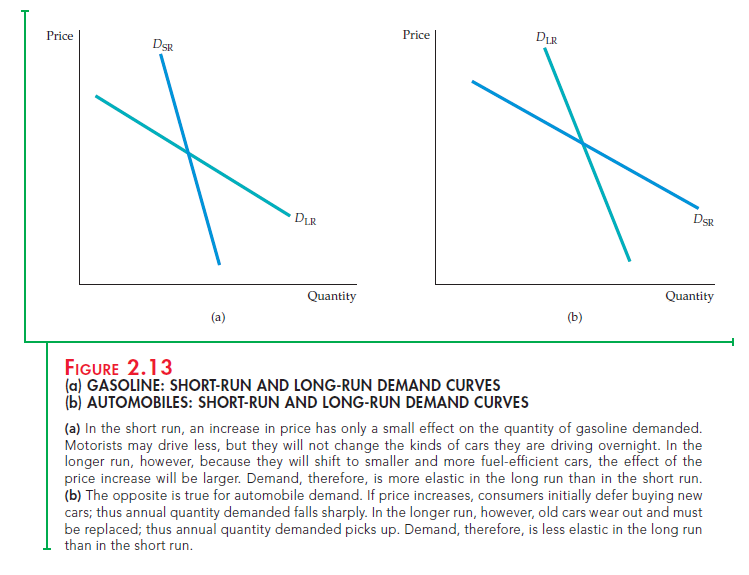
For many goods, demand is much more price elastic in the long run than in the short run. For one thing, it takes time for people to change their consump- tion habits. For example, even if the price of coffee rises sharply, the quantity demanded will fall only gradually as consumers begin to drink less. In addi- tion, the demand for a good might be linked to the stock of another good that changes only slowly. For example, the demand for gasoline is much more elastic in the long run than in the short run. A sharply higher price of gaso- line reduces the quantity demanded in the short run by causing motorists to drive less, but it has its greatest impact on demand by inducing consum- ers to buy smaller and more fuel-efficient cars. But because the stock of cars changes only slowly, the quantity of gasoline demanded falls only slowly. Figure 2.13(a) shows short-run and long-run demand curves for goods such as these.

DEMAND  AND  DURABILITY On the other hand, for some goods just the opposite is true—demand is more elastic in the short run than in the long run. Because these goods (automobiles, refrigerators, televisions, or the capital equip- ment purchased by industry) are durable, the total stock of each good owned by consumers is large relative to annual production. As a result, a small change in the total stock that consumers want to hold can result in a large percentage change in the level of purchases.

Suppose, for example, that the price of refrigerators goes up 10 percent, caus- ing the total stock of refrigerators that consumers want to hold to drop 5 percent. Initially, this will cause purchases of new refrigerators to drop much more than

5 percent. But eventually, as consumers’ refrigerators depreciate (and units must be replaced), the quantity demanded will increase again. In the long run, the total stock of refrigerators owned by consumers will be about 5 percent less than before the price increase. In this case, while the long-run price elasticity of demand for refrigerators would be – .05/.10  =  – 0.5, the short-run elasticity would be much larger in magnitude.

Or consider automobiles. Although annual U.S. demand—new car pur- chases—is about 10 to 12 million, the stock of cars that people own is around

130 million. If automobile prices rise, many people will delay buying new cars. The quantity demanded will fall sharply, even though the total stock of cars that consumers might want to own at these higher prices falls only a small amount. Eventually, however, because old cars wear out and must be replaced, the quantity of new cars demanded picks up again. As a result, the long-run change in the quantity demanded is much smaller than the short- run change. Figure 2.13(b) shows demand curves for a durable good like automobiles.

INCOME ELASTICITIES  Income elasticities also differ from the short run to the long run. For most goods and services—foods, beverages, fuel, entertain- ment, etc.—the income elasticity of demand is larger in the long run than in the short run. Consider the behavior of gasoline consumption during a period of strong economic growth during which aggregate income rises by

10 percent. Eventually people will increase gasoline consumption because they can afford to take more trips and perhaps own larger cars. But this change in consumption takes time, and demand initially increases only by a small amount. Thus, the long-run elasticity will be larger than the short-run elasticity.

For a durable good, the opposite is true. Again, consider automobiles. If aggregate income rises by 10 percent, the total stock of cars that consumers will want to own will also rise—say, by 5 percent. But this change means a much larger increase in current purchases of cars. (If the stock is 130 million, a 5-percent increase is 6.5 million, which might be about 60 to 70 percent of normal demand in a single year.) Eventually consumers succeed in increasing the total number of cars owned; after the stock has been rebuilt, new purchases are made largely to replace old cars. (These new purchases will still be greater than before because a larger stock of cars outstanding means that more cars need to be replaced each year.) Clearly, the short-run income elasticity of demand will be much larger than the long-run elasticity.

CYCLICAL INDUSTRIES Because the demands for durable goods fluctuate so sharply in response to short-run changes in income, the industries that produce these goods are quite vulnerable to changing macroeconomic condi- tions, and in particular to the business cycle—recessions and booms. Thus, these industries are often called cyclical industries—their sales patterns tend to magnify cyclical changes in gross domestic product (GDP) and national income.

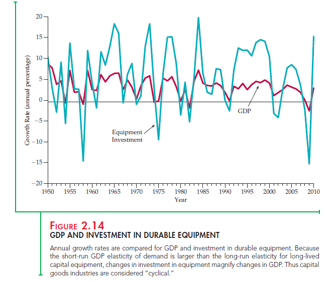
Figures 2.14 and 2.15 illustrate this principle. Figure 2.14 plots two variables over time: the annual real (inflation-adjusted) rate of growth of GDP and the annual real rate of growth of investment in producers’ durable equipment (i.e., machinery and other equipment purchased by firms). Note that although the durable equipment series follows the same pattern as the GDP series, the changes in GDP are magnified. For example, in 1961–1966 GDP grew by at least

4 percent each year. Purchases of durable equipment also grew, but by much more (over 10 percent in 1963–1966). Equipment investment likewise grew much more quickly than GDP during 1993–1998. On the other hand, during the recessions of 1974–1975, 1982, 1991, 2001, and 2008, equipment purchases fell by much more than GDP.

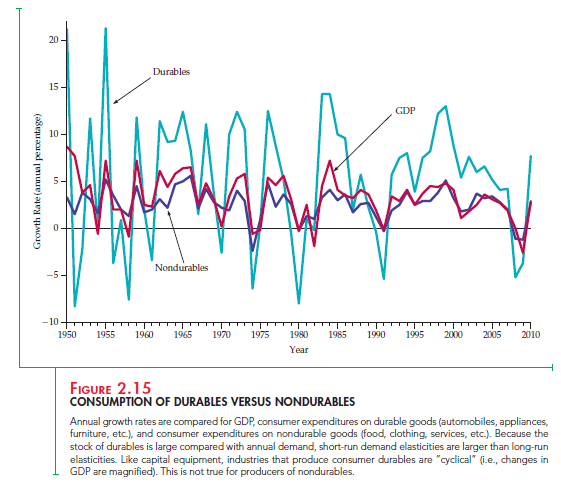
Figure 2.15 also shows the real rate of growth of GDP, along with the annual real rates of growth of spending by consumers on durable goods (automobiles, appliances, etc.) and nondurable goods (food, fuel, clothing, etc.). Note that while both consumption series follow GDP, only the durable goods series tends to magnify changes in GDP. Changes in consumption of nondurables are roughly the same as changes in GDP, but changes in con- sumption of durables are usually several times larger. This is why companies such as General Motors and General Electric are considered “cyclical”: Sales of cars and electrical appliances are strongly affected by changing macroeco- nomic conditions.

2. Supply

Elasticities of supply also differ from the long run to the short run. For most products, long-run supply is much more price elastic than short-run supply: Firms face capacity constraints in the short run and need time to expand capacity by building new production facilities and hiring workers to staff them. This is not to say that the quantity supplied will not increase in the short run if price goes up sharply. Even in the short run, firms can increase output by using their existing facilities for more hours per week, paying workers to work overtime, and hiring some new workers immediately. But firms will be able to expand output much more when they have the time to expand their facilities and hire larger permanent workforces.

For some goods and services, short-run supply is completely inelastic. Rental housing in most cities is an example. In the very short run, there is only a fixed number of rental units. Thus an increase in demand only pushes rents up. In the longer run, and without rent controls, higher rents provide an incentive to renovate existing buildings and construct new ones. As a result, the quantity supplied increases.

For most goods, however, firms can find ways to increase output even in the short run—if the price incentive is strong enough. However, because various constraints make it costly to increase output rapidly, it may require large price increases to elicit small short-run increases in the quantity supplied. We discuss these characteristics of supply in more detail in Chapter 8.

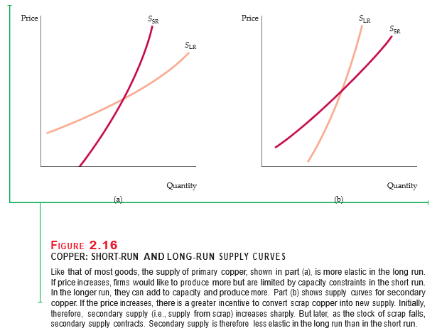
SUPPLY AND DURABILITY For some goods, supply is more elastic in the short run than in the long run. Such goods are durable and can be recycled as part of supply if price goes up. An example is the secondary supply of metals: the supply from scrap metal, which is often melted down and refabricated. When the price of copper goes up, it increases the incentive to convert scrap copper into new supply, so that, initially, secondary supply increases sharply. Eventually, how- ever, the stock of good-quality scrap falls, making the melting, purifying, and refabricating more costly. Secondary supply then contracts. Thus the long-run price elasticity of secondary supply is smaller than the short-run elasticity.

Figures 2.16(a) and 2.16(b) show short-run and long-run supply curves for primary (production from the mining and smelting of ore) and secondary copper production. Table 2.3 shows estimates of the elasticities for each component of supply and for total supply, based on a weighted average of the component elasticities.12  Because secondary supply is only about 20 percent of total supply, the price elasticity of total supply is larger in the long run than in the short run.

Source: Pindyck Robert, Rubinfeld Daniel (2012), Microeconomics, Pearson, 8th edition.