Factors Affecting Optimal Level of Product Availability in a Supply Chain

To understand the factors that influence the optimal level of product availability, consider L. L. Bean, a large mail-order company that sells apparel. One of the products L. L. Bean sells is ski jackets, for which the selling season is from November to February. The buyer at L. L. Bean cur­rently purchases the entire season’s supply of ski jackets from the manufacturer before the start of the selling season. Providing a high level of product availability requires the purchase of a large number of jackets. Although a high level of product availability is likely to satisfy all demand that arises, it is also likely to result in a large number of unsold jackets at the end of the season, with L. L. Bean losing money on unsold jackets. In contrast, a low level of product avail­ability is likely to result in few unsold jackets. However, it is quite likely that L. L. Bean will have to turn away customers who are willing to buy jackets, because they are sold out. In this scenario, L. L. Bean loses potential profit by losing customers. The buyer at L. L. Bean must bal­ance the loss from having too many unsold jackets (if the number of jackets ordered is more than demand) and the lost profit from turning away customers (if the number of jackets ordered is less than demand) when deciding the level of product availability.

The cost of overstocking, denoted by C_o, is the loss incurred by a firm for each unsold unit at the end of the selling season. The cost of understocking, denoted by C_u, is the margin lost by a firm for each lost sale because there is no inventory on hand. The cost of understocking should include the margin lost from current sales, as well as future sales if the customer does not return. In summary, the two key factors that influence the optimal level of product availability are

• Cost of overstocking the product, C_o
• Cost of understocking the product, C_u

We illustrate and develop this relationship in the context of a buying decision at L. L. Bean. The first point to observe is that deciding on an optimal level of product availability makes sense only in the context of demand uncertainty. Traditionally, many firms have forecast a consensus estimate of demand without any measure of uncertainty. In this setting, firms do not make a deci­sion regarding the level of availability; they simply order the consensus forecast. Since the begin­ning of the twenty-first century, firms have developed a better appreciation for uncertainty and have started developing forecasts that include a measure of uncertainty. Incorporating uncer­tainty and deciding on the optimal level of product availability can increase profits relative to using a consensus forecast.

L.L. Bean has a buying committee that decides on the quantity of each product to be ordered. Based on demand over the past few years, the buyers have estimated the demand distri­bution for a women’s red ski parka to be as shown in Table 13-1. This is a deviation from its traditional practice of using the average historical demand as the consensus forecast. To simplify the discussion, we assume that all demand is in hundreds of parkas. The manufacturer also requires that L. L. Bean place orders in multiples of 100. In Table 13-1, p_i is the probability that demand equals D_i, and P_i is the probability that demand is less than or equal to D_i. From Table 13-1, we evaluate the expected demand for parkas as

Under the old policy of ordering the expected value, the buyers would have ordered 1,000 par­kas. However, demand is uncertain, and Table 13-1 shows that there is a 51 percent probability that demand will be 1,000 or less. Thus, a policy of ordering a thousand parkas results in a cycle service level of 51 percent at L. L. Bean. The buying committee must decide on an order size and cycle service level that maximize the profits from the sale of parkas at L. L. Bean.

The loss that L. L. Bean incurs from an unsold parka and the profit that it makes on each parka it sells influences the buying decision. Each parka costs L. L. Bean c = $45 and is priced in the catalog at p = $100. Any unsold parkas at the end of the season are sold at the outlet store for $50. Holding the parka in inventory and transporting it to the outlet store costs L. L. Bean $10. Thus, L. L. Bean recovers a salvage value of 5 = $40 for each parka that is unsold at the end of the season. L. L. Bean makes a profit of p — c = $55 on each parka it sells and incurs a loss of c — s = $5 on each unsold parka that is sold at the outlet store.

The expected profit from ordering 1,000 parkas is given as

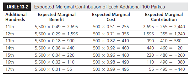
To decide whether to order 1,100 parkas, the buying committee must determine the impact of buying the extra 100 units. If 1,100 parkas are ordered, the extra 100 are sold (for a profit of $5,500) if demand is 1,100 or higher. Otherwise, the extra 100 units are sent to the outlet store at a loss of $500.   From Table 13-1, we see that there is a probability of 0.49 that demand is  1,100 or higher  and a    0.51 probability that demand is 1,000  or less. Thus, we deduce the following:

Expected profit from the extra 100 parkas = 5,500 X Prob( demand > 1,100)

– 500 X Prob(demand < 1,100) = $5,500 X 0.49 — $500 X 0.51 = $2,440

The total expected profit from ordering 1,100 parkas is thus $52,340, which is almost 5 percent higher than the expected profit from ordering 1,000 parkas. Using the same approach, we evaluate the marginal contribution of each additional 100 parkas as in Table 13-2 (see worksheet Table 13-1, 2 in spreadsheet Chapter13-examples). Note that the expected marginal contribution is positive up to 1,300 parkas, but it is negative from that point on. Thus, the optimal order size is 1,300 parkas. From Table 13-2, we have

Expected profit from ordering 1,300 parkas = $49,900 + $2,440 + $1,240 + $580 = $54,160

This is more than an 8 percent increase in profitability relative to the policy of ordering the expected value of 1,000 parkas.

A plot of total expected profits versus the order quantity is shown in Figure 13-1. The opti­mal order quantity maximizes the expected profit. For L. L. Bean, the optimal order quantity is 1,300 parkas, which provides a CSL of 92 percent. Observe that with a CSL of 0.92, L. L. Bean has a fill rate that is much higher. If demand is 1,300 or less, L. L. Bean achieves a fill rate of 100 percent, because all demand is satisfied. If demand is more than 1,300 (say, D), part of the demand (D – 1,300) is not satisfied. In this case, a fill rate of 1,300/D is achieved. Overall, the fill rate achieved at L. L. Bean if 1,300 parkas are ordered is given by

Thus, with a policy of ordering 1,300 parkas, L. L. Bean satisfies, on average, 99 percent of its demand from parkas in inventory.

In the L. L. Bean example, we have a cost of overstocking of C_o = c – s = $5 and a cost of understocking of C_u = p – s = $55. As these costs change, the optimal level of product availability also changes. In the next section, we develop the relationship between the desired CSL and the cost of overstocking and understocking for seasonal items.

1. Optimal Cycle Service Level for Seasonal Items with a single order in a season

In this section, we focus attention on seasonal products such as ski jackets, for which all leftover items must be disposed of at the end of the season. The assumption is that the leftover items from the previous season are not used to satisfy demand for the current season. Assume a retail price per unit of p, a cost of c, and a salvage value of s. We consider the following inputs:

C_o: Cost of overstocking by one unit, C_o = c – s

C_u: Cost of understocking by one unit, C_u = p – c

CSL*: Optimal cycle service level

O*: Corresponding optimal order size

CSL* is the probability that demand during the season will be at or below O*. At the optimal cycle service level CSL^*, the marginal contribution of purchasing an additional unit is zero. If the order quantity is raised from O* to O* + 1, the additional unit sells if demand is larger than O*. This occurs with probability 1 – CSL^* and results in a contribution of p – c. We thus have

Expected benefit of purchasing extra unit = ( 1 – CSL^*) ( p – c)

The additional unit remains unsold if demand is at or below O^*. This occurs with probabil­ity CSL^* and results in a cost of c – s. We thus have

Expected cost of purchasing extra unit = CSL* (c – s)

Thus, the expected marginal contribution of raising the order size from 0* to O* + 1 is given by

(1 – CSL*)(p – c) – CSL*(c – s)

Because the expected marginal contribution must be 0 at the optimal cycle service level, we have

A more rigorous derivation of the previously mentioned formula is provided in Appendix 13A. The optimal CSL* has also been referred to as the critical fractile. The resulting optimal order quan­tity maximizes the firm’s profit. If demand during the season is normally distributed, with a mean of m and a standard deviation of s, the optimal order quantity is given by

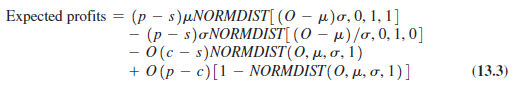
When demand is normally distributed, with a mean of p and a standard deviation of s, the expected profit from ordering O units is given by

The derivation of this formula is provided in Appendix 13B and Appendix 13C. Here, F_S is the standard normal cumulative distribution function and f_S is the standard normal density func­tion discussed in Appendix 12A in Chapter 12. The expected profit from ordering 0 units is evaluated in Excel using Equations 12.22, 12.25, and 12.26, as follows:

Example 13-1 illustrates the use of Equations 13.1 and 13.2 to obtain the optimal cycle ser­vice level and order quantity (see worksheet Example 13-1 in spreadsheet Chapter 13-examples).

EXAMPLE 13-1 Evaluating the Optimal Service Level for Seasonal Items

The manager at Sportmart, a sporting goods store, has to decide on the number of skis to pur­chase for the winter season. Based on past demand data and weather forecasts for the year, management has forecast demand to be normally distributed, with a mean of m = 350 and a standard deviation of s = 100. Each pair of skis costs c = $100 and retails for p = $250. Any unsold skis at the end of the season are disposed of for $85. Assume that it costs $5 to hold a pair of skis in inventory for the season. How many skis should the manager order to maximize expected profits?

Analysis:

In this case, we have

Salvage value = s = $85 – $5 = $80

Cost of understocking = C_u = p – c = $250 – $100 = $150

Cost of overstocking = C_o = c – s = $100 – $80 = $20

Using Equation 13.1, we deduce that the optimal CSL is

Using Equation 13.2, the optimal order size is

Thus, it is optimal for the manager at Sportmart to order 468 pairs of skis, even though the expected number of sales is 350. In this case, because the cost of understocking is much higher than the cost of overstocking, management is better off ordering more than the expected value to cover for the uncertainty of demand.

Using Equation 13.3, the expected profits from ordering O* units are

The expected profit from ordering 350 pairs of skis can be evaluated as $45,718. Thus, ordering 468 pairs results in an expected profit that is almost 8 percent higher than the profit obtained from ordering the expected value of 350 pairs.

When O units are ordered, a firm is left with either too much or too little inventory, depend­ing on demand. When demand is normally distributed, with expected value p and standard devia­tion s, the expected quantity overstocked at the end of the season is given by

The derivation of this formula is provided in Appendix 13D. The formula can be evaluated using Excel as follows:

The expected quantity understocked at the end of the season is given by

The derivation of this formula is provided in Appendix 13E. The formula can be evaluated using Excel as follows:

Example 13-2 illustrates the use of Equations 13.4 and 13.5 to evaluate the quantity expected to be overstocked and understocked as a result of an ordering policy (see worksheet Example 13-2).

EXAMPLE 13-2 Evaluating Expected Overstock and Understock

Demand for skis at Sportmart is normally distributed with a mean of m = 350 and a standard deviation of s = 100. The manager has decided to order 450 pairs of skis for the upcoming season. Evaluate the expected overstock and understock as a result of this policy.

Analysis:

We have an order size O = 450. An overstock results if demand during the season is less than 450. The expected overstock can be obtained using Equation 13.4 as

Thus, the policy of ordering 450 pairs of skis results in an expected overstock of 108 pairs. An understock occurs if demand during the season is higher than 450 pairs. The expected understock can be evaluated using Equation 13.5 as follows:

Thus, the policy of ordering 450 pairs results in an expected understock of 8 pairs. Note that both the expected understock and overstock are positive. This result may seem counterintui­tive, but it makes sense because the values used to calculate an expected understock or overstock are always greater than or equal to zero. For example, if demand is 500 and 450 jackets are in inventory, there is an understock of 50 and an overstock of 0 (not -50). This guarantees that the expected value of each will be greater than or equal to zero.

2. One-Time Orders in the Presence of Quantity Discounts

In this section, we consider a buyer who has to make a single order when the seller offers a price discount based on the quantity purchased. Such a situation may arise in the context of seasonal items such as apparel, for which the manufacturer offers a lower price per unit if order quantities exceed a given threshold. Such decisions also arise at the end of the life cycle for a product or spare parts. Future demand for the product or spare parts is uncertain, and the buyer has a single opportunity to order. The buyer must account for the discount when selecting the order size.

Consider a retailer of spare parts that has one last chance to order parts before the manufac­turer stops production. The part has a retail price per unit of p, a cost to the retailer (without dis­count) of c, and a salvage value of 5. The manufacturer has offered a discounted price of c_d if the retailer orders at least K units. The retailer can make its order size decision using the following steps:

1. Using C_o = c – s and C_u = p – c, evaluate the optimal cycle service level CSL* and order size O* without a discount using Equations 13.1 and 13.2, respectively. Evaluate the expected profit from ordering O* using Equation 13.3.
2. Using C_o  =  c_d – s and C_u  = p – c_d,  evaluate the optimal cycle service level CSL*_d  and order size O* with a discount using Equations 13.1 and 13.2, respectively. If O* > K, evaluate the expected profit from ordering O* units using Equation 13.3. If O*_d < K, evalu­ate the expected profit from ordering K units using Equation 13.3.

3. Order O* units if the profit in step 1 is higher. If the profit in step 2 is higher, order O* units if O* > K or K units if O*_d < K.

We illustrate the procedure in Example 13-3 (see worksheet Example 13-3).

EXAMPLE 13-3 Evaluating Service Level with Quantity Discounts

SparesRUs, an auto parts retailer, must decide on the order size for a 20-year-old model of brakes. The manufacturer plans to discontinue production of these brakes after this last produc­tion run. SparesRUs has forecast remaining demand for the brakes to be normally distributed, with a mean of 150 and a standard deviation of 40. The brakes have a retail price of $200. Any unsold brakes are useless and have no salvage value. The manufacturer plans to sell each brake for $50 if the order is for less than 200 brakes and $45 if the order is for at least 200 brakes. How many brakes should SparesRUs order?

Analysis:

In step 1, we calculate the optimal order quantity at the regular price c = $50:

Cost of understocking = C_u = p  –  c   =    $200 – $50 = $150

Cost of overstocking = C_o = c  –  s   =    $50 – $0 = $50

Using Equation 13.1, we deduce that the optimal CSL is

Using Equation 13.2, the optimal order size is

O* = NORMINV(CSL*, µ, σ) = NORMINV(0.75, 150, 40) = 177

Using Equation 13.3, the expected profit if SparesRUs does not go after the discount is

Expected profit from ordering 177 units = $19,958

In step 2, we consider the discount price cd = $45 and obtain

Cost of understocking = C_u = p –   c_d    =     $200 – $45  = $155

Cost of overstocking = Co = cd – s   =     $45 – $0 =  $45

Using Equation 13.1, we deduce that the optimal CSL with the discount price is

Using Equation 13.2, the optimal order size is

Given that 180 < 200, the retailer must order at least 200 brakes to benefit from the discount. Thus, we calculate the expected profit from ordering 200 units using Equation 13.3 as

Expected profits from ordering 200 units at $45 each = $20,595

It is thus optimal for SparesRUs to order 200 brakes to take advantage of the quantity dis­count. The expected overstock can be calculated using Equation 13.4 to be 52.

3. Desired Cycle Service Level for Continuously Stocked Items

In this section, we focus on products such as detergent that are ordered repeatedly by a retail store such as Walmart. Walmart uses safety inventory to increase the level of avail­ability and decrease the probability of stocking out between successive deliveries. If deter­gent is left over in a replenishment cycle, it can be sold in the next cycle. It does not have to be disposed of at a lower cost. However, a holding cost is incurred as the product is car­ried from one cycle to the next. The manager at Walmart is faced with the issue of deciding the CSL to aim for.

Two extreme scenarios should be considered:

1. All demand that arises when the product is out of stock is backlogged and filled later, when inventories are replenished.
2. All demand arising when the product is out of stock is lost.

The reality in most instances is somewhere in between, with some of the demand lost and other customers returning when the product is in stock. We consider both extreme cases.

We assume that demand per unit time is normally distributed, along with the following inputs:

Q: Replenishment lot size

S: Fixed cost associated with each order

ROP: Reorder point

D: Average demand per unit time

_σD: Standard deviation of demand per unit time

ss: Safety inventory (recall that ss = ROP – D_L)

CSL: Cycle service level C: Unit cost

h: Holding cost as a fraction of product cost per unit time

H: Cost of holding one unit for one unit of time. H = hC

DEMAND DURING STOCKOUT IS BACKLOGGED We first consider the case in which all demand arising when the product is out of stock is backlogged. Because no demand is lost, minimizing costs becomes equivalent to maximizing profits. As an example, consider a Walmart store selling detergent. The store manager offers a rain check at a discount of C_u to each cus­tomer wanting to buy detergent when it is out of stock. Assume that the rain check ensures that all these customers return when inventory is replenished. Thus, C_u is the backlogging or under­stocking cost per unit.

If the store manager increases the level of safety inventory, more orders are satisfied from stock, resulting in lower backlogs. This decreases the backlogging or understocking cost. However, the cost of holding inventory increases. We start by considering the costs and bene­fits of holding an additional unit of safety inventory in each replenishment cycle. If the safety inventory is increased from ss (which provides a cycle service level, CSL) to ss + 1, the sup­ply chain incurs cost to hold the additional unit of inventory for a replenishment cycle (which has duration Q / D). The additional unit of safety inventory is beneficial (the benefit equals the cost of understocking C_u) if demand during the replenishment cycle is such that more than ss units of safety inventory are consumed [this happens with probability (1 – CSL)]. We thus have the following:

Increased cost per replenishment cycle of additional safety inventory of 1 unit = (Q / D)H

Benefit per replenishment cycle of additional safety inventory of 1 unit = (1 – CSL) C_u

In this case, the optimal cycle service level is obtained by equating the additional cost and benefit to be

Given the optimal cycle service level, the required safety inventory can be evaluated using Equation 12.5 if demand is normally distributed.

From Equation 13.6, observe that increasing the lot size Q allows the store manager at Walmart to reduce the cycle service level and, thus, the safety inventory carried. This is because increasing the lot size increases the fill rate and thus reduces the quantity backlogged. One should be careful, however, because an increase in lot size raises the cycle inventory. In general, increas­ing the lot size is not an effective way for a firm to improve product availability.

If the cost of stocking out is known, one can use Equation 13.6 to obtain the appropriate cycle service level (and thus the appropriate level of safety inventory). In many practical set­tings, though, it is hard to estimate the cost of stocking out. In such a situation, a manager may want to evaluate the cost of a stockout implied by the current inventory policy. When a precise cost of stockout cannot be found, this implied stockout cost at least gives an idea of whether inventory should be increased, decreased, or kept about the same. In Example 13-4, we show how Equation 13.6 can be used to impute a cost of stocking out given an inventory policy (see worksheet Examples 13-4,5).

EXAMPLE 13-4 Imputing Cost of Stockout from Inventory Policy

Weekly demand for detergent at Walmart is normally distributed, with a mean of D = 100 gal­lons and a standard deviation of s_D = 20. The replenishment lead time is L = 2 weeks. The store manager at Walmart orders 400 gallons when the available inventory drops to 300 gallons. Each gallon of detergent costs $3. The holding cost Walmart incurs is 20 percent. If all unfilled demand is backlogged and carried over to the next cycle, evaluate the cost of stocking out implied by the current replenishment policy.

Analysis:

In this case, we have

Lot size, Q = 400 gallons

Reorder point, ROP = 300 gallons

Average demand per week, D = 100

Standard deviation of demand per week, σ_D  = 20

Unit cost, C = $3

Holding cost as a fraction of product cost per year, h = 0.2

Cost of holding one unit for one year, H = hC= $0.6

Lead time, L = 2 weeks

We thus have

Mean demand over lead time, DL = DL = 200 gallons

Standard deviation of demand over lead time, σ_L = σ_D √L = 20 √2 = 28.3

Because demand is normally distributed, we can use Equations 12.4 and 12.22 to evaluate the CSL under the current inventory policy:

CSL = F (ROP, DL, σL) = NORMDIST (300, 200, 28.3, 1) = 0.9998

We can thus deduce that the imputed cost of stocking out (using Equation 13.6) is given by

The implication here is that if each shortage of a gallon of detergent costs Walmart $230.77, the current CSL of 0.9998 is optimal. In this particular example, one can claim that the store manager is carrying too much inventory because the cost of stocking out of detergent is unlikely to be $230.77 per gallon.

A manager can use the previous analysis to decide whether the imputed cost of stocking out, and thus the inventory policy, is reasonable.

DEMAND DURING STOCKOUT IS LOST When unfilled demand during the stockout period is lost, the optimal cycle service level CSL^* is given as

We have assumed that Cu is the cost of losing one unit of demand during the stockout period. From comparing Equations 13.6 and 13.7, observe that for the same cost of understock­ing, a supply chain should offer a higher cycle service level if sales are lost rather than back­logged. In Example 13-5, we evaluate the optimal cycle service level if demand is lost during the stockout period (see worksheet Examples 13-4,5).

EXAMPLE 13-5 Evaluating Optimal Service Level When Unmet Demand Is Lost

Consider the situation in Example 13-4 but make the assumption that all demand during a stock­out is lost. Assume that the cost of losing one unit of demand is $2. Evaluate the optimal cycle service level that the store manager at Walmart should target.

Analysis:

In this case, we have

Lot size, Q = 400 gallons

Average demand per year, D = 100 X 52 = 5,200

Cost of holding one unit for one year, H = $0.6

Cost of understocking, Cu = $2

Using Equation 13.7, the optimal cycle service level is given as

The store manager at Walmart should target a cycle service level of 98 percent.

Source: Chopra Sunil, Meindl Peter (2014), Supply Chain Management: Strategy, Planning, and Operation, Pearson; 6th edition.