Production and Cost Theory—A Mathematical Treatment

This appendix presents a mathematical treatment of the basics of production and cost theory. As in the appendix to Chapter 4, we use the method of Lagrange multipliers to solve the firm’s cost-minimizing problem.

1. Cost Minimization

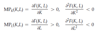
The theory of the firm relies on the assumption that firms choose inputs to the production process that minimize the cost of producing output. If there are two inputs, capital K and labor L, the production function F(K, L) describes the maxi- mum output that can be produced for every possible combination of inputs. We assume that each factor in the production process has positive but decreasing marginal products. Therefore, writing the marginal product of capital and labor as MPK(K, L) and MPL(K, L), respectively, it follows that

A competitive firm takes the prices of both labor w and capital r as given. Then the cost-minimization problem can be written as

Minimize C = wL + rK                                            (A7.1)

subject to the constraint that a fixed output q₀ be produced:

F(K, L) = q0                                       (A7.2)

C represents the cost of producing the fixed level of output q₀.

To determine the firm’s demand for capital and labor inputs, we choose the values of K and L that minimize (A7.1) subject to (A7.2). We can solve this con­strained optimization problem in three steps using the method discussed in the appendix to Chapter 4:

• Step 1: Set up the Lagrangian, which is the sum of two components: the cost of production (to be minimized) and the Lagrange multiplier A times the out­put constraint faced by the firm:

• Step 2: Differentiate the Lagrangian with respect to K, L, and A. Then equate the resulting derivatives to zero to obtain the necessary conditions for a minimum.^[1]

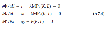
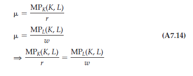
• Step 3: In general, these equations can be solved to obtain the optimizing values of L, K, and A. It is particularly instructive to combine the first two conditions in (A7.4) to obtain

Equation (A7.5) tells us that if the firm is minimizing costs, it will choose its factor inputs to equate the ratio of the marginal product of each factor divided by its price. This is exactly the same condition that we derived as Equation 7.4 (page 247) in the text.

Finally, we can rewrite the first two conditions of (A7.4) to evaluate the Lagrange multiplier:

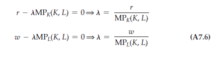
Suppose output increases by one unit. Because the marginal product of capital meas­ures the extra output associated with an additional input of capital, 1/MP_k(K, L) measures the extra capital needed to produce one unit of output. Therefore, r/MP_K(K, L) measures the additional input cost of producing an additional unit of output by increasing capital. Likewise, w/MP_L(K, L) measures the additional cost of producing a unit of output using additional labor as an input. In both cases, the Lagrange multiplier is equal to the marginal cost of production because it tells us how much the cost increases if the amount produced is increased by one unit.

2. Marginal Rate of Technical Substitution

Recall that an isoquant is a curve that represents the set of all input combinations that give the firm the same level of output—say, q₀. Thus, the condition that F(K, L) = q₀ represents a production isoquant. As input combinations are changed along an isoquant, the change in output, given by the total derivative of F(K, L), equals zero (i.e., dq = 0). Thus

It follows by rearrangement that

where MRTS_LK is the firm’s marginal rate of technical substitution between labor and capital.

Now, rewrite the condition given by (A7.5) to get

Because the left side of (A7.8) represents the negative of the slope of the iso­quant, it follows that at the point of tangency of the isoquant and the isocost line, the firm’s marginal rate of technical substitution (which trades off inputs while keeping output constant) is equal to the ratio of the input prices (which represents the slope of the firm’s isocost line).

We can look at this result another way by rewriting (A7.9):

Equation (A7.10) is the same as (A7.5) and tells us that the marginal products of all production inputs must be equal when these marginal products are adjusted by the unit cost of each input.

3. Duality in Production and Cost Theory

As in consumer theory, the firm’s input decision has a dual nature. The opti­mum choice of K and L can be analyzed not only as the problem of choosing the lowest isocost line tangent to the production isoquant, but also as the prob­lem of choosing the highest production isoquant tangent to a given isocost line. Suppose we wish to spend C₀ on production. The dual problem asks what com­bination of K and L will let us produce the most output at a cost of C₀. We can see the equivalence of the two approaches by solving the following problem:

We can solve this problem using the Lagrangian method:

• Step 1: We set up the Lagrangian

where p is the Lagrange multiplier.

• Step 2: We differentiate the Lagrangian with respect to K, L, and o and set the resulting equation equal to zero to find the necessary conditions for a maximum:

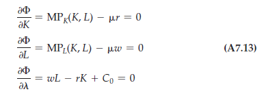
• Step 3: Normally, we can use the equations of (A7.13) to solve for K and In particular, we combine the first two equations to see that

This is the same result as (A7.5)—that is, the necessary condition for cost minimization.

4. The Cobb-Douglas Cost and Production Functions

Given a specific production function F(K, L), conditions (A7.13) and (A7.14) can be used to derive the cost function C(q). To understand this principle, let’s work through the example of a Cobb-Douglas production function. This production function is

where A, a, and b are positive constants.

We assume that a < 1 and b < 1, so that the firm has decreasing marginal products of labor and capital.^[2] If a + b = 1, the firm has constant returns to scale, because doubling K and L doubles F. If a + b > 1, the firm has increasing returns to scale, and if a + b < 1, it has decreasing returns to scale.

As an application, consider the carpet industry described in Example 6.4 (page 221). The production of both small and large firms can be described by Cobb- Douglas production functions. For small firms, a = .77 and b = .23. Because a + b = 1, there are constant returns to scale. For larger firms, however, a = .83 and b = .22. Thus a + b = 1.05, and there are increasing returns to scale. The Cobb-Douglas production function is frequently encountered in economics and can be used to model many kinds of production. We have already seen how it can accommodate differences in returns to scale. It can also account for changes in technology or productivity through changes in the value of A: The larger the value of A, more can be produced for a given level of K and L.

To find the amounts of capital and labor that the firm should utilize to mini­mize the cost of producing an output q₀, we first write the Lagrangian

Differentiating with respect to L, K, and A, and setting those derivatives equal to 0, we obtain

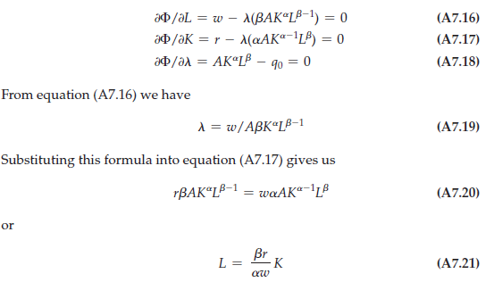
(A7.21) is the expansion path. Now use Equation (A7.21) to substitute for L in equation (A7.18):

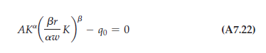
We can rewrite the new equation as:

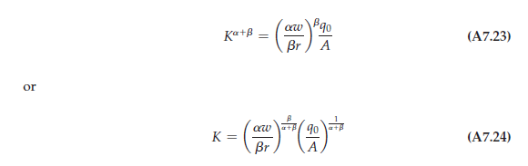
(A7.24) is the factor demand for capital. We have now determined the cost-min­imizing quantity of capital: Thus, if we wish to produce q₀ units of output at least cost, (A7.24) tells us how much capital we should employ as part of our production plan. To determine the cost-minimizing quantity of labor, we simply substitute equation (A7.24) into equation (A7.21):

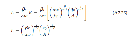
(A7.25) is the constrained factor demand for labor. Note that if the wage rate w rises relative to the price of capital r, the firm will use more capital and less labor. Suppose that, because of technological change, A increases (so the firm can produce more output with the same inputs); in that case, both K and L will fall.

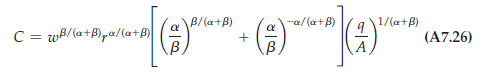
This cost function tells us (1) how the total cost of production increases as the level of output q increases, and (2) how cost changes as input prices change. When a + b equals 1, equation (A7.26) simplifies to
We have shown how cost-minimization subject to an output constraint can be used to determine the firm’s optimal mix of capital and labor. Now we will determine the firm’s cost function. The total cost of producing any output q can be obtained by substituting equations (A7.24) for K and (A7.25) for L into the equation C = wL + rK. After some algebraic manipulation we find that

In this case, therefore, cost will increase proportionately with output. As a result, the production process exhibits constant returns to scale. Likewise, if a + b is greater than 1, there are increasing returns to scale; if a + b is less than 1, there are decreasing returns to scale.

The firm’s cost function contains many desirable features. To appreciate this fact, consider the special constant returns to scale cost function (A7.27). Suppose that we wish to produce q₀ in output but are faced with a doubling of the wage. How should we expect our costs to change? New costs are given by

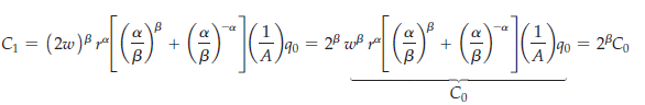
Recall that at the beginning of this section, we assumed that a < 1 and fi < 1. Therefore, C₁ < 2C₀. Even though wages doubled, the cost of producing q₀ less than doubled. This is the expected result. If a firm suddenly had to pay more for labor, it would substitute away from labor and employ more of the relatively cheaper capital, thereby keeping the increase in total cost in check.

Now consider the dual problem of maximizing the output that can be pro­duced with the expenditure of C₀ dollars. We leave it to you to work through this problem for the Cobb-Douglas production function. You should be able to show that equations (A7.24) and (A7.25) describe the cost-minimizing input choices. To get you started, note that the Lagrangian for this dual problem is $ = AK^aL^b – o(wL + rK – C₀).

Source: Pindyck Robert, Rubinfeld Daniel (2012), Microeconomics, Pearson, 8th edition.