Projections

We have looked at methods to determine cycles in market data. We now look at how we can use the knowledge about cycles in the data to project the next low and perhaps the next high.

1. Projecting Period

To project the time for the next low, we need three facts: the period length of the cycle of interest, the standard error of that cycle, and the ideal starting point from which to measure it into the future. In the example, we have found periods of 34 days and 17 days. Because we only have four cycles of the 34-day period, we cannot determine accurate projections. However, for the 17-day cycle, we have plenty of examples with apparently little error.

The first and most simple method is to use a ruler or the paper trick mentioned previously to draw points on the chart that match the periods determined from measurement. This is subject to interpretive error; in our example, the process suggested a 17-day cycle that was borne out by further analysis.

Second, we could use the vertical line shown on the charts and project into the future. This method is accurate once we know the precise cycle periods from our analysis and the beginning point. However, it does not estimate an error range of when to expect the next turning point.

Third, we could use a linear regression model of the periods to estimate the period, the error, and the exact location for the starting point (Kirkpatrick, 1990). To begin this process, we identify the lows given by the ratio in Figure 19.14, beginning numbering with 1. Thus, the first low, which occurred on December 8, 2010, would be 1; the second low, occurring on December 31, would be 2; and so forth. Table 19.2 displays this numbering of lows under the Number column heading.

TABLE 19.2 Kirkpatrick Linear Method of Determining the Optimal Location of Cycle Period Lows

In addition, each time interval is converted to a sequence of whole numbers to eliminate the problem of weekends and to make calculation easier. In our example, for instance, the first 18-day low occurred on October 14. We record that as low Number 1 at time interval 0 because it is the beginning of our period. The next low occurred on November 7. Because this low occurred 16.63 trading days after low Number 1, we would label it low Number 2 and with a day number 16.63 days. (In other words, it occurred 16.63 days after low Number 1.) These numbers result from converting calendar days to trading days with the factor 4.85/7 trading days per calendar days. From now on, all days will be measured from low Number 1. The third low occurred on December 2. We would label it low Number 3 with a period of 33.95 days from low Number 1. The time interval for all lows is measured from the first low. Successive lows are entered into the spreadsheet in a similar manner until the end of the period is reached, as shown in Table 19.2.

This process creates three columns in the spreadsheet. The first column is the low’s specific number, the independent variable. The second is the low’s corresponding date. The third is the number of calendar days from the previous low. The fourth column is the calendar day converted to a trading day. The fifth is the cumulative numbers of each trading day low.

We then use linear regression to determine a best fit between the low numbers (1, 2, 3, and so on) and the time interval (in trading days) on which it occurred. The results of the linear regression suggest that the cycle period is 17.89 days, or roughly 18 days.

Using these numbers, we can project future lows in column six. The best projection into the future is for the next 18-day low (Number 11) to occur 17.738 days after the model’s estimate of the tenth low. As illustrated in Figure 19.15, this suggests a Number 11 projected low will occur at time interval 178.199, or on June 28, and the Number 12 projected low will occur on July 24 plus or minus a day or so. As it turns out, the longer 34-day cycle is due for a low around July 25.

2. Projecting Amplitude

Figure 19.15 also shows how amplitude can vary enormously. Indeed, the variation is so large that prediction is almost impossible. We can only conjecture what the future might bring in amplitude because, so far, no reasonable and consistent method exists. In this example, what can help in amplitude projection, however, is the concept of nesting. Cycles tend to oscillate within cycles. Thus, their outer boundaries, as defined by envelopes, can give us a rough estimate of what to expect for amplitude. Again, let us look at our same data example, this time shown in Figure 19.16 with a 34-day cycle envelope.

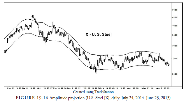
We project the next cycle lows using the linear regression method outlined previously. This gives us an idea of when to expect cycle lows and, by inference, cycle highs. We know that the low around early June is a 34- day low. Because the May low was the second 34-day low since major low in January, we also know that the May low is likely one of a larger cycle that is influencing the shorter cycles. It is, therefore, a powerful low and likely of the 70-80 day variety, and we should expect the immediately following cycles to translate right. The problem is that the current price is below the May low already and the shorter cycles are translating left already. Thus, if the May low was of a higher order, the longer-term cycle is turning downward.

Left translation has already occurred in the first 17-day cycle and likely has occurred in the first 34-day cycle. If so, while a 34-day low is due soon, the following 34-day cycle could break below the January low and result in a market decline into September or October, the next time for a 70-80 day low.

3. Half-Cycle Reversal

We mentioned earlier that the half-cycle, centered, moving average represents the full cycle under investigation. When the half-cycle, centered, SMA reverses, it signals that the low in the cycle of interest has occurred. Because the half-cycle, centered, moving average is plotted half its cycle back from the present, it represents what the full cycle was doing 1/4 of a cycle length back. Thus, if the full cycle is bottoming as represented by the centered moving average, we know that the full cycle still has 3/4 of its time and perhaps distance to travel. An ideal cycle will spend half its time rising and half its time declining. At 1/4 the time through the cycle, we know that it has another 1/4 to go before showing signs of downward reversal. It is, thus, halfway through its advance. Being so, we can take the distance that it has traveled and assume that the price will approximately double what it did during the first quarter. We now have an estimate of the potential amplitude of the current full cycle. Of course, the amplitude also depends on the next higher order cycle. If that longer cycle is rising, we can assume the projection will be exceeded as the cycle translates to the right, and if the next higher is downward, we likely will not see an upward reversal in the centered moving average. If the next higher cycle is flat, the projection should be precise. The bottom line, then, is when one-quarter of a cycle is completed, we can begin to see what the potential shape of the full cycle will be from looking at the behavior of the half-cycle, centered moving average.

4. The FLD and Centered Moving Average Crossovers (the “Forward Line”)

Hurst describes another interesting method of projecting prices in a cycle called the FLD line. FLD stands for Future Line of Demarcation. It is the closing prices projected a half-cycle period forward from the current price. In Figure 19.17, for example, the cycle of interest is the 34-day cycle. Projecting closing prices a half-cycle forward, or 17 days, produces the FLD line. Several observations can be made.

First, because the projection is a half-cycle forward, its peak should appear when a low is expected and vice versa. This is because prices should rise during the first half into a cycle measured from the cycle low and should decline during the second half. Thus, the FLD high should occur at the same time as the real cycle low and vice versa. Of course, this can be upset by the influence of the next longer cycle. If prices peak after the low in the FLD, or bottom before the top in the FLD, the underlying trend is upward. Conversely, if prices bottom after the FLD peak or peak before the FLD peak, the underlying trend is downward. The location of the FLD can, thus, help us with determining the trend of the next longer cycle.

In Figure 19.17, in October, the peak in the FLD and the bottom in prices coincide precisely. In February, a price peak was suggested by the bottoming of the FLD. In late November, prices pay no attention to the FLD peak and continue downward, suggesting that by the next cycle low, prices will be considerably lower.

Second, by representing a half-cycle, the FLD line is declining when the cycle prices are advancing. The crossover of current prices through the FLD should occur at roughly the midpoint both timewise and pricewise in the advance or decline. In Figure 19.17, the downward crossover of prices through the FLD in late September at $40.14 projected a decline of $6.29 to an estimated target of $33.85. The bottom closing price at the actual low was $30.57, almost 3 ^lh points lower than projected. This overshoot of the projected low is evidence that the higher order cycle is declining. On the rally after that low, the projected target was $43.23, yet the spike and one-day reversal high was at 42.25, this time short of the target. When downward targets are exceeded and upward targets not reached, the implication is that the underlying trend has turned downward. Indeed, shortly after this failed attempt on the upside, the price tumbled for several months. The rule, then, is that when prices exceed the upper FLD target price after the crossover, the next higher-order cycle is strong in the direction of the price crossover. Conversely, if prices do not reach their target, or as in some cases, do not cross the FLD line, the next higher-order cycle is weak.

Third, the FLD can act as support or resistance. This is not so noticeable in the example because half the action was in a trading range and the other half in a steady decline. If prices halt at the FLD and reverse, the underlying cycle trend is not reversing on schedule. It will increase in strength in its original direction. If prices penetrate the FLD, the cycle is still intact, and prices will head for the midpoint target. Depending on whether it reaches that target or overruns it will then give clues as to the strength of the next longer cycle trend. It is, therefore, important to watch price action when it reaches the FLD to see if it is confirming the strength or weakness of the cycle direction.

Because the FLD line follows price action exactly, it can give an erratic appearance and make crossovers somewhat arbitrary, based on only one or two days’ action. To combat this, analysts will project forward the half-cycle SMA in the same manner as the FLD. This gives a smoothed line, called the forward line, that is easier to work with. The same rules for the FLD apply to the forward line.

5. The Tillman Method

Jim Tillman (1990) of Cycletrend, Inc. developed a number of methods for cycle projections. He used centered moving averages of half-cycles after he determined the dominant cycle periods.

Tillman’s analysis concentrates on what he calls focal points. Focal points occur when three or more half-cycle, centered, moving averages cross at roughly the same location. In Figure 19.18, crossovers of two half-cycle moving averages (17-day and 34-day) are shown rather than three, for clarity.

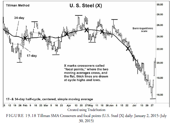
One observation is that focal points occur at roughly the halfway point of cycle advances or declines. Notice the thick horizontal lines at the 18-day cycle peaks, the troughs, and the Xs at the crossovers in Figure 19.18. The crossovers occur roughly halfway between the peak and trough in points. The practical problem
from this observation is that by the time the lagging half-cycle moving averages have crossed, prices have already reached their projection. The crossover, thus, occurs when the cycle is ending its run up or down. When you see a crossover in an upward leg of a cycle, you know that the upward leg is about to peak or already has.

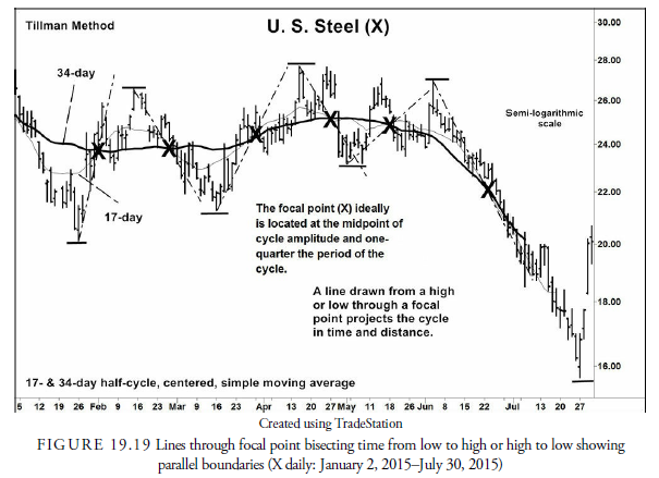
In Figure 19.19, lines are drawn from the high or low of a cycle through the focal point. The upward sloping lines will continue through to the high of the cycle, and the downward sloping lines will continue through to the low of the cycle. The time from the low (high) to the focal point will equal, approximately, the time to that high (low), as will the distance. In our example in Figure 19.19, in February, the time from the cycle low to the focal point was 8 days, and 7 days later, the peak was reached. In March-April, the rally through the focal point took 11 days. The price reached its high for the cycle in 10 days. The crossover is the center of the cosine wave. It is the center in time as well as distance.

If we then draw a trend line between two successive focal points (X), we have an estimate of the direction of the next higher-order cycle. Lines drawn parallel to that trend line to the immediate highs and lows will show that the trend is roughly midway between the parallel lines and that they represent the boundaries of the cycle (see Figure 19.20). The advantage of using these parallel lines formed from the trend between focal points is that they can be projected into the future, whereas the moving average parallel lines had to be drawn freehand as a guess.

When the parallel lines are decisively broken, we know that the next higher-order cycle has changed direction. For example, in Figure 19.20, the parallel lower line from the connection between the last two focal points was penetrated in early June. In addition, the rallies fell short of the upper bound projected from the same focal points. This is bearish behavior for the next higher cycle. It also makes sense because the parallel lines define the boundaries of the lower-order cycle. If they are broken, it must be due to the change in direction of the next higher-order cycle.

6. Concept of Commonality

Another of Hurst’s principles, that of “commonality,” suggested that issues of the same nature tend to have the same cycles but with different amplitudes. In the stock market, this principle implies that individual stocks will have generally the same cycles as the stock market averages. The study of cycles requires the analyst’s close attention and analysis. Few analysts pursue it because the conversion of the analysis to computers is difficult and requires some knowledge of applied mathematics and trigonometry. Much of the analysis must be done by hand. Because cycle analysis is intensive and subjective, the analyst must select stocks with sufficient volatility such that the cycles of interest will have enough amplitude to become profitable if correctly timed. The same can be said of commodities in that innate volatility is a factor that should be considered when selecting an issue to trade using cycle analysis.

Source: Kirkpatrick II Charles D., Dahlquist Julie R. (2015), Technical Analysis: The Complete Resource for Financial Market Technicians, FT Press; 3rd edition.