Periods of Four Years or Less in Technical Analysis

A day is a definite period of time. A year, within small limits, is also definite. A month, however, may be lunar or solar; it may also be a number of other things. Hence 40 months of our present calendar must remain an approximation and certainly not an exact measure of the duration of cycles, if, as we shall be led to believe, natural phenomena have some part in determining the pattern of their recurrence. (Smith, 1939, p. 20)

1. Four-Year or Presidential Cycle

As Figure 9.5 shows, when the stock market peaks and declines, the earlier rise and subsequent decline are quick and steep, with advances averaging 12 months, but often lasting much longer, and declines averaging only 6 months. These devastating declines are the reason for the study of market timing. Market timing would save a lot of agony if it was successful. At first market technicians looked at the periodicity of market peaks because they were generally easy to define. And in doing so, they found the interesting phenomena is that while the peaks don’t show any cyclicality, the bottoms do. Bottoms tend to occur every four years with a reasonable statistical variance.

Wesley C. Mitchell (1874—1948), economics professor and one of the founders of the National Bureau of Economic Research (NBER), was the originator of the 40-month cycle theory. He empirically discovered that the U.S. economy from 1796-1923 suffered a recession, on average and excluding four wars, every 40 months, or approximately every four years.

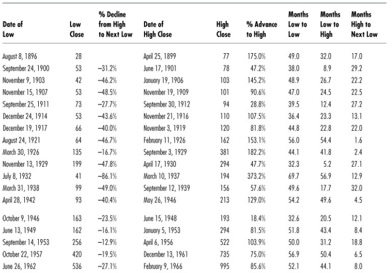
Today, the four-year cycle, from price bottom to price bottom, is the most widely accepted and most easily recognized cycle in the stock market. Occasionally it strays from four years, but only by a portion of a year (see Figure 9.6). This is a remarkably consistent series.

Almost all cycles are measured from bottom to bottom. Tops fail to occur as regularly, but, of course, their average interval is also four years (see Table 9.2). Some analysts have argued that because the U.S. Presidential elections are also four years apart, the cycle is due to the election cycle (see the next section, “Election Year Pattern”). It is, thus, often called the “Presidential cycle.” However, this cycle also occurs in countries that do not have four-year elections, such as Great Britain. It may be that U.S. economic strength is so huge and so globally powerful that other countries are forced to follow its stock market cycles, or it may be that the 40- month (almost four years) economic cycle Wesley Mitchell discovered 80 years ago is still dominant but has been slightly stretched by economic and the Federal Reserve policy action. Whatever the reason for its existence, the four-year cycle is obviously a very strong, important, and reliable cycle.

2. Election Year Pattern

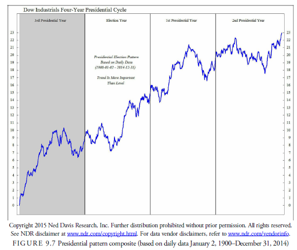
Yale Hirsch, editor of the Stock Trader’s Almanac (www.stocktradersalmanac.com), has compiled statistics on the four-year cycle many call the U .S. Presidential election cycle and broken it down into the characteristics that have occurred each year for the period that a President is in office. Since 1832, the market has risen a total of 557% during the last two years of each administration and only 81% during the first two years. This amounts to an average of 13.6% per year for each of the last two years of an administration and only 2.0% for each of the first two years. Indeed, since 1965, none of the 13 major lows occurred in the fourth year of a presidency, and more than half (9) occurred in the second year. Hirsh’s presumption is that the incumbent party wants to appear in a favorable light during the last two years, and especially in the last year of an administration, to be reelected. To do this, aside from providing the normal “spin” about their accomplishments, they force interest rates lower and stimulate the economy. At least, history shows that interest rates are inversely correlated with the stock market during those latter two years. How the administration in power can force them lower is subject to conjecture.

In any case, this is a reasonable and relatively consistent pattern (see Figure 9.7). Some would argue that it is confusing “cause” with “correlation” and that there may not be a direct causal link between politics and the stock market. Such an argument can be made about many occurrences in nature and in man that appear to cause the stock market to react. The human mind often requires an explanation for stock market behavior. It will invent causal relationships where they do not exist. This mental tendency is something for the technical analyst to be mindful of and is the primary reason that concentration always should be focused on price action rather than on speculating about what might or might not be the cause for its behavior.

3. Seasonal Patterns

A seasonal pattern in agricultural prices has been known for centuries. More recently, interest rates have followed a seasonal pattern as money was borrowed for seed and returned when the crops were gathered. It turns out that seasonality exists in almost all economic statistics, and most producers of economic statistics, such as the Treasury, Federal Reserve, National Bureau of Economic Research, The Conference Board, and many others, adjust their numbers for seasonality. Technical analysts sometimes frown upon this practice because it distorts real figures with adjusted figures. However, it is an admission that seasonality is an important factor in economic statistics and that the earth’s tilt and travel around its orbit have a substantial effect on prices, markets, and economic activity.

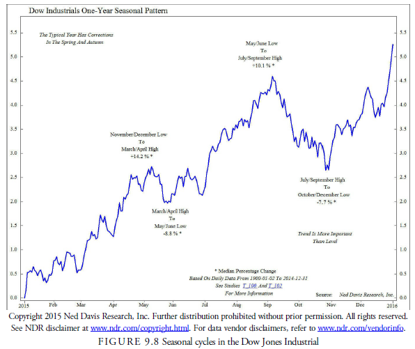
The U.S. Treasury bond market has seasonal tendencies. In Figure 9.8, the performance by month of Treasury bonds is averaged to show that the latter part of the year is the strongest period for the bond market, whereas the winter through spring is the weakest. This means that long-term interest rates, which travel inversely to bond prices, will tend to decline in the summer and fall and rise in the winter and spring.

In the commodity markets, such products as corn, hogs, and oil are those most affected by seasonality. However, changes are occurring in the seasonality in the agricultural sector because many food products are now produced in and shipped from the southern hemisphere in the “off-season.” However, “seasonal” does not mean that from a trading or investment standpoint, a position should be held for many months. In oil, for example, since 1983, the best performance months are July through September, and the weakest is usually October (“Futures Insight: Crude Oil,” Active Trader Magazine, July 2004, p. 70). In orange juice contracts, for example, a seasonal trade for 35 years has been 74% profitable for short trades initiated on June 4 and closed on July 1 (Momsen, 2004). Almost all commodity and stocks have seasonal components that, once recognized, can be profitable. This is called entry date/exit date trading. Price action at or near each date should be analyzed closely because dates are only arbitrary, but once a seasonal pattern is recognized, with proper discipline and observation, it can be profitable over time.

“Sell in May and go away” (usually until October 1) refers to the tendency for the stock market to decline from May to September and rise from October to April. In the past ten years, August and September have been the worst months for performance, and October, November, and January have the best gains, with another small rise in April. According to this model, May is the month to sell, and August is the month to start looking for a bottom. This model has been very consistent. Notice in Table 9.2 that 17 out of 30, or 57%, of the four-year cycle bottoms occurred in September, October, November, or December. Only one peak has occurred in October since 1896. Only one peak has occurred in August, and only four have happened in September. No peaks have occurred in January. In other words, in stock prices, there seems to be a downward bias in the late spring and summer and an upward bias in the late fall and winter. In a study by Active Trader Magazine (“May-October System, The Trading System Lab,” Active Trader Magazine, July 2003, p. 42), the results of buying on October 1 and selling short on May 15 for ten years, January 1993 through March 2003, showed excellent results. The only problem was the occurrence of large drawdowns on the short side during the speculative bubble in 1997 and 1998. The recovery from such drawdowns was quick, however, and the possibility of another speculative bubble in the immediate future is remote. Thus, this simple seasonal system seems to have merit, even if it is only used as a guide as to when to be aggressive and when to be cautious.

Source: Kirkpatrick II Charles D., Dahlquist Julie R. (2015), Technical Analysis: The Complete Resource for Financial Market Technicians, FT Press; 3rd edition.