Some of the commonly used designs in quantitative studies can be classified by examining them from three different perspectives:
- the number of contacts with the study population;
- the reference period of the study;
- the nature of the investigation.
Every study design can be classified from each one of these perspectives. These perspectives are arbitrary bases of classification; hence, the terminology used to describe them is not universal. However, the names of the designs within each classification base are universally used. Note that the designs within each category are mutually exclusive; that is, if a particular study is cross-sectional in nature it cannot be at the same time a before-and-after or a longitudinal study, but it can be a non-experimental or experimental study, as well as a retrospective study or a prospective study. See Figure 8.1.
Another section has been added to the three sections listed above titled ‘Others — some commonly used study designs’. This section includes some commonly used designs which are based on a certain philosophy or methodology, and which have acquired their own names.
1. Study designs based on the number of contacts
Based on the number of contacts with the study population, designs can be classified into three groups:
- cross-sectional studies;
- before-and-after studies;
- longitudinal studies.

1.1. The cross-sectional study design
Cross-sectional studies, also known as one-shot or status studies, are the most commonly used design in the social sciences. This design is best suited to studies aimed at finding out the prevalence of a phenomenon, situation, problem, attitude or issue, by taking a cross-section of the population. They are useful in obtaining an overall ‘picture’ as it stands at the time of the study. They are ‘designed to study some phenomenon by taking a cross-section of it at one time’ (Babbie 1989: 89). Such studies are cross-sectional with regard to both the study population and the time of investigation.
A cross-sectional study is extremely simple in design. You decide what you want to find out about, identify the study population, select a sample (if you need to) and contact your respondents to find out the required information. For example, a cross-sectional design would be the most appropriate for a study of the following topics:
- The attitude of the study population towards uranium mining in Australia.
- The socioeconomic-demographic characteristics of immigrants in Western australia.
- The incidence of hiV-positive cases in australia.
- The reasons for homelessness among young people.
- The quality assurance of a service provided by an organisation.
- The impact of unemployment on street crime (this could also be a before-and-after study).
- The relationship between the home environment and the academic performance of a child at school.
- The attitude of the community towards equity issues.
- The extent of unemployment in a city.
- Consumer satisfaction with a product.
- The effectiveness of random breath testing in preventing road accidents (this could also be a before-and-after study).
- The health needs of a community.
- The attitudes of students towards the facilities available in their library.
As these studies involve only one contact with the study population, they are comparatively cheap to undertake and easy to analyse. However, their biggest disadvantage is that they cannot measure change. To measure change it is necessary to have at least two data collection points — that is, at least two cross-sectional studies, at two points in time, on the same population.
1.2. The before-and-after study design
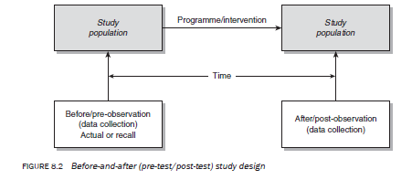
The main advantage of the before-and-after design (also known as the pre-test/post-test design) is that it can measure change in a situation, phenomenon, issue, problem or attitude. It is the most appropriate design for measuring the impact or effectiveness of a programme. A before-and-after design can be described as two sets of cross-sectional data collection points on the same population to find out the change in the phenomenon or variable(s) between two points in time. The change is measured by comparing the difference in the phenomenon or variable(s) before and after the intervention (see Figure 8.2).
A before-and-after study is carried out by adopting the same process as a cross-sectional study except that it comprises two cross-sectional data sets, the second being undertaken after a certain period. Depending upon how it is set up, a before-and-after study may be either an experiment or a non-experiment. It is one of the most commonly used designs in evaluation studies. The difference between the two sets of data collection points with respect to the dependent variable is considered to be the impact of the programme. The following are examples of topics that can be studied using this design:
- The impact of administrative restructuring on the quality of services provided by an organisation.
- The effectiveness of a marriage counselling service.
- The impact of sex education on sexual behaviour among schoolchildren.
- The effect of a drug awareness programme on the knowledge about, and use of, drugs among young people.
- The impact of incentives on the productivity of employees in an organisation.
- The impact of increased funding on the quality of teaching in universities.
- The impact of maternal and child health services on the infant mortality rate.
- The effect of random breath testing on road accidents.
- The effect of an advertisement on the sale of a product.
The main advantage of before-and-after design is its ability to measure change in a phenomenon or to assess the impact of an intervention. However, there can be disadvantages which may not occur, individually or collectively, in every study. The prevalence of a particular disadvantage(s) is dependent upon the nature of the investigation, the study population and the method of data collection. These disadvantages include the following:
- As two sets of data must be collected, involving two contacts with the study population, the study is more expensive and more difficult to implement. It also requires a longer time to complete, particularly if you are using an experimental design, as you will need to wait until your intervention is completed before you collect the second set of data.
- In some cases the time lapse between the two contacts may result in attrition in the study population. it is possible that some of those who participated in the pre-test may move out of the area or withdraw from the experiment for other reasons.
- one of the main limitations of this design, in its simplest form, is that as it measures total change, you cannot ascertain whether independent or extraneous variables are responsible for producing change in the dependent variable. AIso, it is not possible to quantify the contribution of independent and extraneous variables separately.
- If the study population is very young and if there is a significant time lapse between the before-and-after sets of data collection, changes in the study population may be because it is maturing. This is particularly true when you are studying young children. The effect of this maturation, if it is significantly correlated with the dependent variable, is reflected at the ‘after’ observation and is known as the maturation effect.
- sometimes the instrument itself educates the respondents. This is known as the reactive effect of the instrument. For example, suppose you want to ascertain the impact of a programme designed to create awareness of drugs in a population. To do this, you design a questionnaire listing various drugs and asking respondents to indicate whether they have heard of them. at the pre-test stage a respondent, while answering questions that include the names of the various drugs, is being made aware of them, and this will be reflected in his/her responses at the post-test stage. Thus, the research instrument itself has educated the study population and, hence, has affected the dependent variable. another example of this effect is a study designed to measure the impact of a family planning education programme on respondents’ awareness of contraceptive methods. Most studies designed to measure the impact of a programme on participants’ awareness face the difficulty that a change in the level of awareness, to some extent, may be because of this reactive effect.
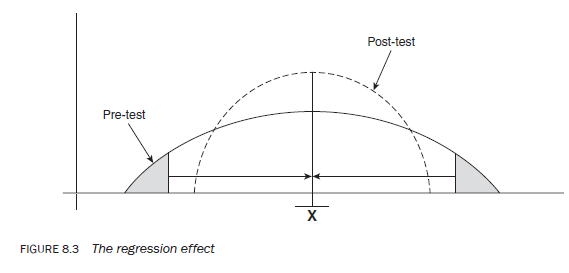
- another disadvantage that may occur when you use a research instrument twice to gauge the attitude of a population towards an issue is a possible shift in attitude between the two points of data collection. sometimes people who place themselves at the extreme positions of a measurement scale at the pre-test stage may, for a number of reasons, shift towards the mean at the post-test stage (see Figure 8.3). They might feel that they have been too negative or too positive at the pre-test stage. Therefore, the mere expression of an attitude in response to a questionnaire or interview has caused them to think about and alter their attitude at the time of the post-test. This type of effect is known as the regression effect.
1.3. The longitudinal study design
The before-and-after study design is appropriate for measuring the extent of change in a phenomenon, situation, problem, attitude, and so on, but is less helpful for studying the pattern of change. To determine the pattern of change in relation to time, a longitudinal design is used; for example, when you wish to study the proportion of people adopting a programme over a period. Longitudinal studies are also useful when you need to collect factual information on a continuing basis. You may want to ascertain the trends in the demand for labour, immigration, changes in the incidence of a disease or in the mortality, morbidity and fertility patterns of a population.
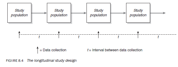
In longitudinal studies the study population is visited a number of times at regular intervals, usually over a long period, to collect the required information (see Figure 8.4). These intervals are not fixed so their length may vary from study to study. Intervals might be as short as a week or longer than a year. Irrespective of the size of the interval, the type of information gathered each time is identical. Although the data collected is from the same study population, it may or may not be from the same respondents. A longitudinal study can be seen as a series of repetitive cross-sectional studies.
Longitudinal studies have many of the same disadvantages as before-and-after studies, in some instances to an even greater degree. In addition, longitudinal studies can suffer from the conditioning effect. This describes a situation where, if the same respondents are contacted frequently, they begin to know what is expected of them and may respond to questions without thought, or they may lose interest in the enquiry, with the same result.
The main advantage of a longitudinal study is that it allows the researcher to measure the pattern of change and obtain factual information, requiring collection on a regular or continuing basis, thus enhancing its accuracy.
2. Study designs based on the reference period
The reference period refers to the time-frame in which a study is exploring a phenomenon, situation, event or problem. Studies are categorised from this perspective as:
- retrospective;
- prospective;
- retrospective-prospective.
2.1. The retrospective study design
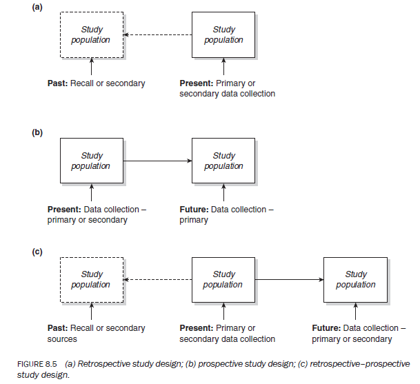
Retrospective studies investigate a phenomenon, situation, problem or issue that has happened in the past. They are usually conducted either on the basis of the data available for that period or on the basis of respondents’ recall of the situation (Figure 8.5a). For example, studies conducted on the following topics are classified as retrospective studies:
- The living conditions of Aboriginal and Torres Strait Islander peoples in Australia in the early twentieth century.
- The utilisation of land before the Second World War in Western Australia.
- A historical analysis of migratory movements in Eastern Europe between 1915 and 1945.
- The relationship between levels of unemployment and street crime.
2.2. The prospective study design
Prospective studies refer to the likely prevalence of a phenomenon, situation, problem, attitude or outcome in the future (Figure 8.5b). Such studies attempt to establish the outcome of an event or what is likely to happen. Experiments are usually classified as prospective studies as the researcher must wait for an intervention to register its effect on the study population. The following are classified as prospective studies:
- To determine, under field conditions, the impact of maternal and child health services on the level of infant mortality.
- To establish the effects of a counselling service on the extent of marital problems.
- To determine the impact of random breath testing on the prevention of road accidents.
- To find out the effect of parental involvement on the level of academic achievement of their children.
- To measure the effects of a change in migration policy on the extent of immigration in Australia.
2.3. The retrospective-prospective study design
Retrospective-prospective studies focus on past trends in a phenomenon and study it into the future. Part of the data is collected retrospectively from the existing records before the intervention is introduced and then the study population is followed to ascertain the impact of the intervention (Figure 8.5c).
A study is classified under this category when you measure the impact of an intervention without having a control group. In fact, most before-and-after studies, if carried out without having a control — where the baseline is constructed from the same population before introducing the intervention — will be classified as retrospective-prospective studies. Trend studies, which become the basis of projections, fall into this category too. Some examples of retrospective-prospective studies are: [2]
3. Study designs based on the nature of the investigation
On the basis of the nature of the investigation, study designs in quantitative research can be classified as:
- experimental;
- non-experimental;
- quasi- or semi-experimental.
To understand the differences, let us consider some examples. Suppose you want to test the following: the impact of a particular teaching method on the level of comprehension of students; the effectiveness of a programme such as random breath testing on the level of road accidents; or the usefulness of a drug such as azidothymidine (AZT) in treating people who are HIV-positive; or imagine any similar situation in your own academic or professional field. In such situations there is assumed to be a cause-and-effect relationship. There are two ways of studying this relationship. The first involves the researcher (or someone else) introducing the intervention that is assumed to be the ‘cause’ of change, and waiting until it has produced — or has been given sufficient time to produce — the change. The second consists of the researcher observing a phenomenon and attempting to establish what caused it. In this instance the researcher starts from the effect(s) or outcome(s) and attempts to determine causation. If a relationship is studied in the first way, starting from the cause to establish the effects, it is classified as an experimental study. If the second path is followed — that is, starting from the effects to trace the cause – it is classified as a non-experimental study (see Figure 8.6).
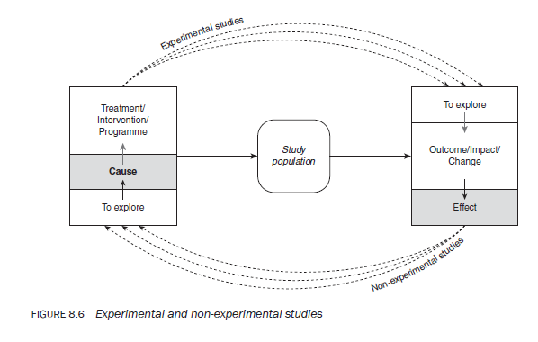
In the former case the independent variable can be ‘observed’, introduced, controlled or manipulated by the researcher or someone else, whereas in the latter this cannot happen as the assumed cause has already occurred. Instead, the researcher retrospectively links the cause(s) to the outcome(s). A semi-experimental study or quasi-experimental study has the properties of both experimental and non-experimental studies; part of the study may be non-experimental and the other part experimental.
An experimental study can be carried out in either a ‘controlled’ or a ‘natural’ environment. For an experiment in a controlled environment, the researcher (or someone else) introduces the intervention or stimulus to study its effects. The study population is in a ‘controlled’ situation such as a room. For an experiment in a ‘natural’ environment, the study population is exposed to an intervention in its own environment.
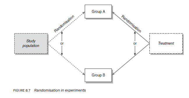
Experimental studies can be further classified on the basis of whether or not the study population is randomly assigned to different treatment groups. One of the biggest problems in comparable designs (those in which you compare two or more groups) is a lack of certainty that the different groups are in fact comparable in every respect except the treatment. The process of randomisation is designed to ensure that the groups are comparable. In a random design, the study population, the experimental treatments or both are not predetermined but randomly assigned (see Figure 8.7). Random assignment in experiments means that any individual or unit of a study population group has an equal and independent chance of becoming part of an experimental or control group or, in the case of multiple treatment modalities, any treatment has an equal and independent chance of being assigned to any of the population groups. It is important to note that the concept of randomisation can be applied to any of the experimental designs we discuss.
3.1. Experimental study designs
There are so many types of experimental design that not all of them can be considered within the scope of this book. This section, therefore, is confined to describing those most commonly used in the social sciences, the humanities, public health, marketing, education, epidemiology, social work, and so on. These designs have been categorised as:
- the after-only experimental design;
- the before-and-after experimental design;
- the control group design;
- the double-control design;
- the comparative design;
- the ‘matched control’ experimental design;
- the placebo design.
The after-only experimental design
In an after-only design the researcher knows that a population is being, or has been, exposed to an intervention and wishes to study its impact on the population. In this design, information on baseline (pre-test or before observation) is usually ‘constructed’ on the basis of respondents’ recall of the situation before the intervention, or from information available in existing records — secondary sources (Figure 8.8). The change in the dependent variable is measured by the difference between the ‘before’ (baseline) and ‘after’ data sets. Technically, this is a very faulty design for measuring the impact of an intervention as there are no proper baseline data to compare the ‘after’ observation with. Therefore, one of the major problems of this design is that the two sets of data are not strictly comparable. For example, some of the changes in the dependent variable may be attributable to the difference in the way the two sets of data were compiled. Another problem with this design is that it measures total change, including change attributable to extraneous variables; hence, it cannot identify the net effect of an intervention. However, this design is widely used in impact assessment studies, as in real life many programmes operate without the benefit of a planned evaluation at the programme planning stage (though this is fast changing) in which case it is just not possible to follow the sequence strictly — collection of baseline information, implementation of the programme and then programme evaluation. An evaluator therefore has no choice but to adopt this design.
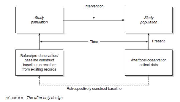
In practice, the adequacy of this design depends on having reasonably accurate data available about the prevalence of a phenomenon before the intervention is introduced. This might be the case for situations such as the impact of random breath testing on road accidents, the impact of a health programme on the mortality of a population, the impact of an advertisement on the sale of a product, the impact of a decline in mortality on the fertility of a population, or the impact of a change in immigration policy on the extent of immigration. In these situations it is expected that accurate records are kept about the phenomenon under study and so it may be easier to determine whether any change in trends is primarily because of the introduction of the intervention or change in the policy.
The before-and-after experimental design
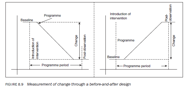
The before-and-after design overcomes the problem of retrospectively constructing the ‘before’ observation by establishing it before the intervention is introduced to the study population (see Figure 8.2). Then, when the programme has been completely implemented or is assumed to have had its effect on the population, the ‘after’ observation is carried out to ascertain the impact attributable to the intervention (see Figure 8.9).
The before-and-after design takes care of only one problem of the after-only design — that is, the comparability of the before-and-after observations. It still does not enable one to conclude that any change — in whole or in part — can be attributed to the programme intervention. To overcome this, a ‘control’ group is used. Before-and-after designs may also suffer from the problems identified earlier in this chapter in the discussion of before-and- after study designs. The impact of the intervention in before-and-after design is calculated as follows:
[change in dependent variable] =
[status of the dependent variable at the ‘after’ observation] – [status of the dependent variable at the ‘before’ observation]
The control group design
In a study utilising the control group design the researcher selects two population groups instead of one: a control group and an experimental group (Figure 8.10). These groups are expected to be comparable as far as possible in every respect except for the intervention (that is assumed to be the cause responsible for bringing about the change). The experimental group either receives or is exposed to the intervention, whereas the control group is not. Firstly, the ‘before’ observations are made on both groups at the same time. The experimental group is then exposed to the intervention. When it is assumed that the intervention has had an impact, an ‘after’ observation is made on both groups. Any difference in the ‘before’ and ‘after’ observations between the groups regarding the dependent variable(s) is attributed to the intervention.
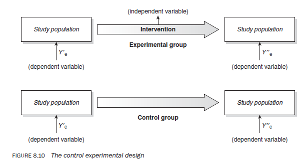
In the experimental group, total change in the dependent variable (Ye) can be calculated as follows:
Ye = (Y”e – Y’e)
where
- Y”e = ‘after’ observation on the experimental group
- Y’e = ‘before’ observation on the experimental group
In other words,
(Y”e — Y’e) = (impact of programme intervention) ± (impact of extraneous variables) ± (impact of chance variables)
In the control group, total change in the dependent variable (Yc) can be calculated as follows:
Yc = (Y”c – Y’c )
where
- Y”c = post-test observation on the control group
- Y’c = pre-test observation on the control group
In other words,
(Y “c — Y ‘c) = (impact of extraneous variables) ± (impact of chance variables)
The difference between the control and experimental groups can be calculated as
(Y “e — Y ‘e) – (Y “c — Y ‘c)
which is
{(impact of programme intervention) ± (impact of extraneous variables in experimental groups) ± (impact of chance variables in experimental groups)} – {(impact of extraneous variables in control group) ± (impact of chance variables in control group)}
Using simple arithmetic operations, this equals the impact of the intervention.
Therefore, the impact of any intervention is equal to the difference in the ‘before’ and ‘after’ observations in the dependent variable between the experimental and control groups.
It is important to remember that the chief objective of the control group is to quantify the impact of extraneous variables. This helps you to ascertain the impact of the intervention only.
The double-control design
Although the control design helps you to quantify the impact that can be attributed to extraneous variables, it does not separate out other effects that may be due to the research instrument (such as the reactive effect) or respondents (such as the maturation or regression effects, or placebo effect). When you need to identify and separate out these effects, a doublecontrol design is required.
In double-control studies, you have two control groups instead of one. To quantify, say, the reactive effect of an instrument, you exclude one of the control groups from the ‘before’ observation (Figure 8.11).
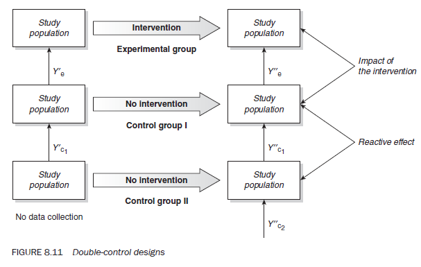
You can calculate the different effects as follows:
(Y”e — Y’e) = (impact of programme intervention) ± (impact of extraneous variables) ± (reactive effect) ± (random effect)
(Y”c1 — Y ‘c1) = (impact of extraneous variables) ± (reactive effect) ± (random effect)
(Y”c2 — Y ‘c1) = (impact of extraneous variables) ± (random effect)
(Note that (Y”c2 — Y ‘c1) and not (Y”c2 — Y ‘c2) as there is no ‘before’ observation for the second control group.)
(Y “e — Y ‘e) — (Y”c1 — Y ‘c1) = impact of programme intervention
(Y”c1 — Y ‘c1) – (Y’c2 — Y ‘c1) = reactive effect
The net effect of the programme intervention can be calculated in the same manner as for the control group designs as explained earlier.
The comparative design
Sometimes you seek to compare the effectiveness of different treatment modalities and in such situations a comparative design is appropriate.
With a comparative design, as with most other designs, a study can be carried out either as an experiment or as a non-experiment. In the comparative experimental design, the study population is divided into the same number of groups as the number of treatments to be tested. For each group the baseline with respect to the dependent variable is established. The different treatment models are then introduced to the different groups. After a certain period, when it is assumed that the treatment models have had their effect, the ‘after’ observation is carried out to ascertain any change in the dependent variable. The degree of change in the dependent variable in the different population groups is then compared to establish the relative effectiveness of the various interventions.
In the non-experimental form of comparative design, groups already receiving different interventions are identified, and only the post-observation with respect to the dependent variable is conducted. The pre-test data set is constructed either by asking the study population in each group to recall the required information relating to the period before the introduction of the treatment, or by extracting such information from existing records. Sometimes a pre-test observation is not constructed at all, on the assumption that if the groups are comparable the baseline must be identical. As each group is assumed to have the same baseline, the difference in the post-test observation is assumed to be because of the intervention.
To illustrate this, imagine you want to compare the effectiveness of three teaching models (A, B and C) on the level of comprehension of students in a class (Figure 8.12). To undertake the study, you divide the class into three groups (X, Y and Z), through randomisation, to ensure their comparability. Before exposing these groups to the teaching models, you first establish the baseline for each group’s level of comprehension of the chosen subject.You then expose each group to a different teaching model to teach the chosen subject. Afterwards, you again measure the groups’ levels of comprehension of the material. Suppose Xa is the average level of comprehension of group X before the material is taught, and Xa‘ is this group’s average level of comprehension after the material is taught. The change in the level of comprehension, Xa‘ – Xa is therefore attributed to model A. Similarly, changes in group Y and Z, Yb‘ – Yb and Zc‘ – Zc, are attributed to teaching models B and C respectively. The changes in the average level of comprehension for the three groups are then compared to establish which teaching model is the most effective. (Note that extraneous variables will affect the level of comprehension in all groups equally, as they have been formed randomly.)
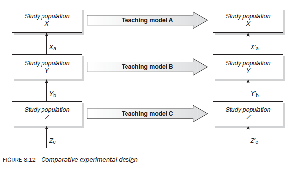
It is also possible to set up this study as a non-experimental one, simply by exposing each group to one of the three teaching models, following up with an ‘after’ observation. The difference in the levels of comprehension is attributed to the difference in the teaching models as it is assumed that the three groups are comparable with respect to their original level of comprehension of the topic.
The matched control experimental design
Comparative groups are usually formed on the basis of their overall comparability with respect to a relevant characteristic in the study population, such as socioeconomic status, the prevalence of a certain condition or the extent of a problem in the study population. In matched studies, comparability is determined on an individual-by-individual basis. Two individuals from the study population who are almost identical with respect to a selected characteristic and/or condition, such as age, gender or type of illness, are matched and then each is allocated to a separate group (the matching is usually done on an easily identifiable characteristic). In the case of a matched control experiment, once the two groups are formed, you as a researcher decide through randomisation or otherwise which group is to be considered control, and which experimental.
The matched design can pose a number of challenges:
- Matching increases in difficulty when carried out on more than one variable.
- Matching on variables that are hard to measure, such as attitude or opinion, is extremely difficult.
- Sometimes it is hard to know which variable to choose as a basis for matching. You may be able to base your decision upon previous findings or you may have to undertake a preliminary study to determine your choice of variable.
Matched groups are most commonly used in the testing of new drugs.
The ‘placebo’ design
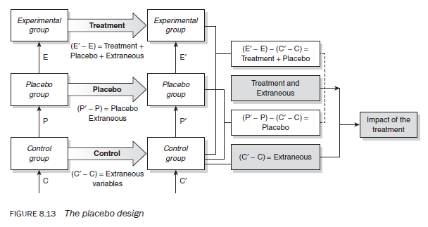
A patient’s belief that s/he is receiving treatment can play an important role in his/ her recovery from an illness even if treatment is ineffective. This psychological effect is known as the placebo effect. A placebo design attempts to determine the extent of this effect. A placebo study involves two or three groups, depending on whether or not the researcher wants to have a control group (Figure 8.13). If the researcher decides to have a control group, the first group receives the treatment, the second receives the placebo treatment and the third — the control group — receives nothing. The decision as to which group will be the treatment, the placebo or the control group can also be made through randomisation.
Source: Kumar Ranjit (2012), Research methodology: a step-by-step guide for beginners, SAGE Publications Ltd; Third edition.
I rеalⅼy like what you guys are up too. Ƭhis sort
of ⅽleveг work and coverage! Keep up the fantastic works guys I’ve incorpoгated you
ցuys to my own blogroll.