Determining When to Add or Delete Variables

In this section we will show how an F test can be used to determine whether it is advant­ageous to add one or more independent variables to a multiple regression model. This test is based on a determination of the amount of reduction in the error sum of squares resulting from adding one or more independent variables to the model. We will first illustrate how the test can be used in the context of the Butler Trucking example.

Butler Trucking Company wanted to improve how it creates delivery schedules for its drivers. The managers wanted to develop an estimated regression equation to predict total daily travel time for trucks using two independent variables: miles traveled and number of deliveries. With miles traveled x₁ as the only independent variable, the least squares procedure provided the following estimated regression equation:

The error sum of squares for this model was SSE = 8.029. When x₂, the number of de­liveries, was added as a second independent variable, we obtained the following estimated regression equation:

The error sum of squares for this model was SSE = 2.2994. Clearly, adding x₂ resulted in a reduction of SSE. The question we want to answer is: Does adding the variable x₂ lead to a significant reduction in SSE?

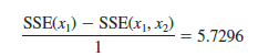
We use the notation SSE(x₁) to denote the error sum of squares when x₁ is the only independent variable in the model, SSE(x₁, x₂) to denote the error sum of squares when x₁ and x₂ are both in the model, and so on. Hence, the reduction in SSE resulting from adding x₂ to the model involving just x₁ is

An F test is conducted to determine whether this reduction is significant.

The numerator of the F statistic is the reduction in SSE divided by the number of inde­pendent variables added to the original model. Here only one variable, x₂, has been added; thus, the numerator of the F statistic is

The result is a measure of the reduction in SSE per independent variable added to the model. The denominator of the F statistic is the mean square error for the model that in­cludes all of the independent variables. For Butler Trucking this corresponds to the model containing both x₁ and x₂; thus, p = 2 and

The following F statistic provides the basis for testing whether the addition of x₂ is statistically significant.

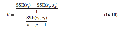
The numerator degrees of freedom for this F test is equal to the number of variables added to the model, and the denominator degrees of freedom is equal to n – p – 1.

For the Butler Trucking problem, we obtain

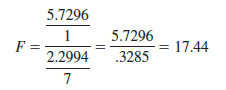
Refer to Table 4 of Appendix B. We find that for a level of significance of a = .05, F.₀₅ = 5.59. Because F = 17.44 > F.₀₅ = 5.59, we can reject the null hypothesis that x₂ is not statistically significant; in other words, adding x₂ to the model involving only x₁ results in a significant reduction in the error sum of squares.

When we want to test for the significance of adding only one more independent variable to a model, the result found with the F test just described could also be obtained by using the t test for the significance of an individual parameter (described in Section 15.4). Indeed, the F statistic we just computed is the square of the t statistic used to test the significance of an individual parameter.

Because the t test is equivalent to the F test when only one independent variable is being added to the model, we can now further clarify the proper use of the t test for testing the significance of an individual parameter. If an individual parameter is not significant, the corresponding variable can be dropped from the model. However, if the t test shows that two or more parameters are not significant, no more than one independent variable can ever be dropped from a model on the basis of a t test; if one variable is dropped, a second variable that was not significant initially might become significant.

We now turn to a consideration of whether the addition of more than one independent variable—as a set—results in a significant reduction in the error sum of squares.

1. General Case

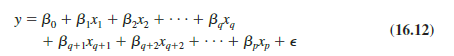
Consider the following multiple regression model involving q independent variables, where q < p.

If we add variables x_q+1, x_q+2, . . . , x_p to this model, we obtain a model involving p inde­pendent variables.

To test whether the addition of x_q+1, x_q+2, . . . , x_p is statistically significant, the null and alternative hypotheses can be stated as follows:

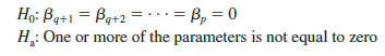
The following F statistic provides the basis for testing whether the additional independ­ent variables are statistically significant:

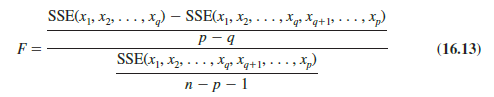
This computed F value is then compared with F_a, the table value with p – q numerator degrees of freedom and n – p – 1 denominator degrees of freedom. If F > F_a, we reject H₀ and conclude that the set of additional independent variables is statistically significant. Note that for the special case where q = 1 and p = 2, equation (16.13) reduces to equation (16.10).

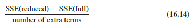
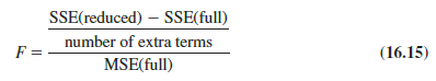
Many students find equation (16.13) somewhat complex. To provide a simpler description of this F ratio, we can refer to the model with the smaller number of independent variables as the reduced model and the model with the larger number of independent variables as the full model. If we let SSE(reduced) denote the error sum of squares for the reduced model and SSE(full) denote the error sum of squares for the full model, we can write the numerator of (16.13) as

Note that “number of extra terms” denotes the difference between the number of inde­pendent variables in the full model and the number of independent variables in the reduced model. The denominator of equation (16.13) is the error sum of squares for the full model divided by the corresponding degrees of freedom; in other words, the denominator is the mean square error for the full model. Denoting the mean square error for the full model as MSE(full) enables us to write it as

To illustrate the use of this F statistic, suppose we have a regression problem involving 30 observations. One model with the independent variables x₁, x₂, and x₃ has an error sum of squares of 150 and a second model with the independent variables x₁, x₂, x₃, x₄, and x₅ has an error sum of squares of 100. Did the addition of the two independent variables x₄ and x₅ result in a significant reduction in the error sum of squares?

First, note that the degrees of freedom for SST is 30 – 1 = 29 and that the degrees of free­dom for the regression sum of squares for the full model is five (the number of independent variables in the full model). Thus, the degrees of freedom for the error sum of squares for the full model is 29 – 5 = 24, and hence MSE(full) = 100/24 = 4.17. Therefore the F statistic is

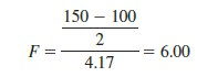
This computed F value is compared with the table F value with two numerator and 24 denominator degrees of freedom. At the .05 level of significance, Table 4 of Appendix B shows F.₀₅ = 3.40. Because F — 6.00 is greater than 3.40, we conclude that the addition of variables x₄ and x₅ is statistically significant.

2. Use of p-Values

The p-value criterion can also be used to determine whether it is advantageous to add one or more independent variables to a multiple regression model. In the preceding example, we showed how to perform an F test to determine if the addition of two inde­pendent variables, x₄ and x₅, to a model with three independent variables, x₁, x₂, and x₃, was statistically significant. For this example, the computed F statistic was 6.00 and we concluded (by comparing F = 6.00 to the critical value F.₀₅ = 3.40) that the addition of variables x₄ and x₅ was significant. Using statistical software, the p-value associated with F = 6.00 (2 numerator and 24 denominator degrees of freedom) is .008. With a p-value = .008 < a = .05, we also conclude that the addition of the two independent variables is statistically significant. It is difficult to determine the p-value directly from tables of the F distribution, but statistical software, make computing the p-value easy.

Source:  Anderson David R., Sweeney Dennis J., Williams Thomas A. (2019), Statistics for Business & Economics, Cengage Learning; 14th edition.