Suppose we collected data for one dependent variable y and k independent variables x1, x2, . . . , xk. Our objective is to use these data to develop an estimated regression equation that provides the best relationship between the dependent and independent variables. As a general framework for developing more complex relationships among the independent variables, we introduce the concept of a general linear model involving p independent variables.
In equation (16.1), each of the independent variables Zj (where j = 1, 2, . . . , p) is a function of x1, x2, . . . , xk (the variables for which data are collected). In some cases, each Zj may be a function of only one x variable. The simplest case is when we collect data for just one variable x1 and want to predict y by using a straight-line relationship. In this case z1 = x1 and equation (16.1) becomes
![]()
In the statistical modeling literature, equation (16.2) is called a simple first-order model with one predictor variable.
1. Modeling Curvilinear Relationships
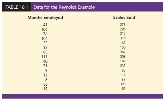
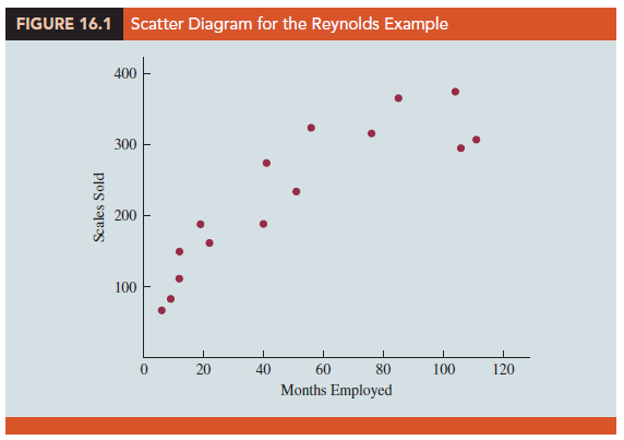
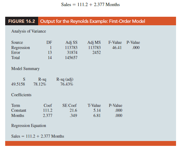
More complex types of relationships can be modeled with equation (16.1). To illustrate, let us consider the problem facing Reynolds, Inc., a manufacturer of industrial scales and laboratory equipment. Managers at Reynolds want to investigate the relationship between length of employment of their salespeople and the number of electronic laboratory scales sold. Table 16.1 gives the number of scales sold by 15 randomly selected salespeople for the most recent sales period and the number of months each salesperson has been employed by the firm. Figure 16.1 is the scatter diagram for these data. The scatter diagram indicates a possible curvilinear relationship between the length of time employed and the number of units sold. Before considering how to develop a curvilinear relationship for Reynolds, let us consider the output in Figure 16.2 corresponding to a simple first-order model; the estimated regression is
where
Sales = number of electronic laboratory scales sold
Months = the number of months the salesperson has been employed
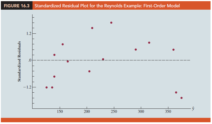
Figure 16.3 is the corresponding standardized residual plot. Although the computer output shows that the relationship is significant (p-value = .000) and that a linear relationship explains a high percentage of the variability in sales (R-sq = 78.12%), the standardized residual plot suggests that a curvilinear relationship is needed.
To account for the curvilinear relationship, we set z1 = x1 and z2 = x2 in equation (16.1) to obtain the model
![]()
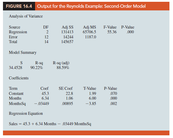
This model is called a second-order model with one predictor variable. To develop an estimated regression equation corresponding to this second-order model, the statistical software package we are using needs the original data in Table 16.1, as well as that data corresponding to adding a second independent variable that is the square of the number of months the employee has been with the firm. In Figure 16.4 we show the output corresponding to the second-order model; the estimated regression equation is
Sales = 45.3 + 6.34 Months – .03449 MonthsSq
where
MonthsSq = the square of the number of months the salesperson has been employed
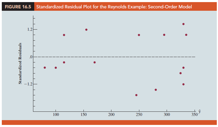
Figure 16.5 is the corresponding standardized residual plot. It shows that the previous curvilinear pattern has been removed. At the .05 level of significance, the computer output shows that the overall model is significant (p-value for the F test is .000); note also that the p-value corresponding to the t-ratio for MonthsSq (p-value = .002) is less than .05, and hence we can conclude that adding MonthsSq to the model involving Months is significant. With R-sq(adj) = 88.59%, we should be pleased with the fit provided by this estimated regression equation. More important, however, is seeing how easy it is to handle curvilinear relationships in regression analysis.
Clearly, many types of relationships can be modeled by using equation (16.1). The regression techniques with which we have been working are definitely not limited to linear, or straight-line, relationships. In multiple regression analysis the word linear in the term “general linear model” refers only to the fact that b0, b1, … , bp all have exponents of 1; it does not imply that the relationship between y and the xi,s is linear. Indeed, in this section we have seen one example of how equation (16.1) can be used to model a curvilinear relationship.
2. Interaction
If the original data set consists of observations for y and two independent variables x1 and x2, we can develop a second-order model with two predictor variables by setting z1 = x1, z2 = x2, z3 = x²1, z4 = 4 and z5 = x1x2 in the general linear model of equation (16.1). The model obtained is
![]()
In this second-order model, the variable z5 = x1x2 is added to account for the potential effects of the two variables acting together. This type of effect is called interaction.
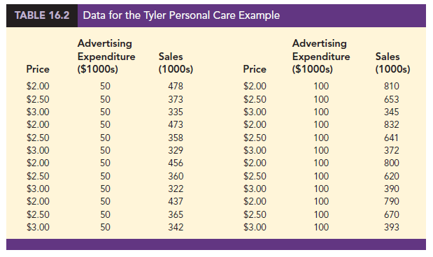
To provide an illustration of interaction and what it means, let us review the regression study conducted by Tyler Personal Care for one of its new shampoo products. Two factors believed to have the most influence on sales are unit selling price and advertising expenditure. To investigate the effects of these two variables on sales, prices of $2.00, $2.50, and $3.00 were paired with advertising expenditures of $50,000 and $100,000 in 24 test markets. The unit sales (in thousands) that were observed are reported in Table 16.2.
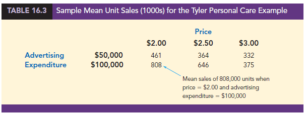
Table 16.3 is a summary of these data. Note that the sample mean sales corresponding to a price of $2.00 and an advertising expenditure of $50,000 is 461,000, and the sample mean sales corresponding to a price of $2.00 and an advertising expenditure of $100,000 is 808,000. Hence, with price held constant at $2.00, the difference in the sample mean sales between advertising expenditures of $50,000 and $100,000 is 808,000 – 461,000 = 347,000 units. When the price of the product is $2.50, the difference in the sample mean sales is 646,000 – 364,000 = 282,000 units. Finally, when the price is $3.00, the difference in the sample mean sales is 375,000 – 332,000 = 43,000 units. Clearly, the difference in the sample mean sales between advertising expenditures of $50,000 and $100,000 depends on the price of the product. In other words, at higher selling prices, the effect of increased advertising expenditure diminishes. These observations provide evidence of interaction between the price and advertising expenditure variables.
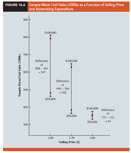
To provide another perspective of interaction, Figure 16.6 shows the sample mean sales for the six price-advertising expenditure combinations. This graph also shows that the effect of advertising expenditure on the sample mean sales depends on the price of the product; we again see the effect of interaction. When interaction between two variables is present, we cannot study the effect of one variable on the response y independently of the other variable. In other words, meaningful conclusions can be developed only if we consider the joint effect that both variables have on the response.
To account for the effect of interaction, we will use the following regression model:
Note that equation (16.5) reflects Tyler’s belief that the number of units sold depends linearly on selling price and advertising expenditure (accounted for by the β1x1 and β2x 2 terms), and that there is interaction between the two variables (accounted for by the β3x1x2 term).
To develop an estimated regression equation, a general linear model involving three independent variables (z1, z2, and z3) was used.
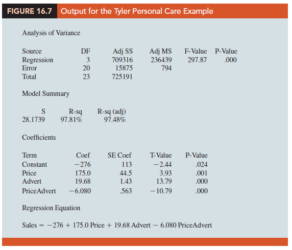
Figure 16.7 is the output corresponding to the interaction model for the Tyler Personal Care example. The resulting estimated regression equation is
Sales = -276 1 175 Price 1 19.68 Advert – 6.08 PriceAdvert
where
Sales = unit sales (1000s)
Price = price of the product ($)
Advert = advertising expenditure ($1000s)
PriceAdvert = interaction term (Price times Advert)
Because the model is significant (p-value for the F test is .000) and the p-value corresponding to the t test for PriceAdvert is .000, we conclude that interaction is significant given the linear effect of the price of the product and the advertising expenditure. Thus, the regression results show that the effect of advertising expenditure on sales depends on the price.
3. Transformations Involving the Dependent Variable
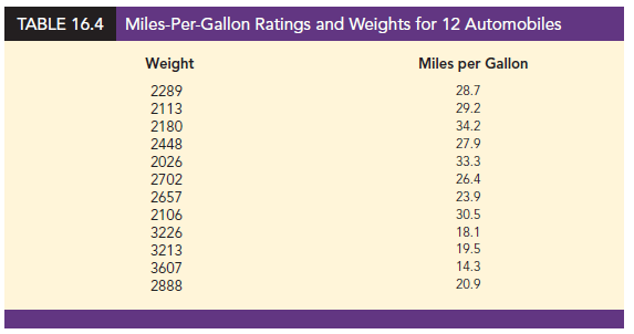
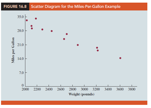
In showing how the general linear model can be used to model a variety of possible relationships between the independent variables and the dependent variable, we have focused attention on transformations involving one or more of the independent variables. Often it is worthwhile to consider transformations involving the dependent variable y. As an illustration of when we might want to transform the dependent variable, consider the data in Table 16.4, which shows the miles-per-gallon ratings and weights for 12 automobiles. The scatter diagram in Figure 16.8 indicates a negative linear relationship between these two variables. Therefore, we use a simple first-order model to relate the two variables. The output is shown in Figure 16.9; the resulting estimated regression equation is
MPG = 56.1 – .011644 Weight
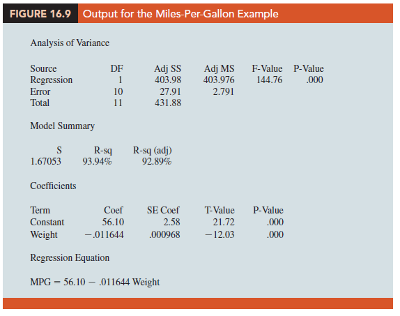
where
MPG = miles-per-gallon rating
Weight = weight of the car in pounds
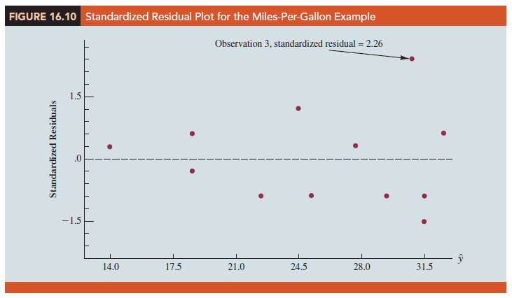
The model is significant (p-value for the F test is .000) and the fit is very good (R-sq = 93.54%). However, inspecting the standardized residual plot in Figure 16.10, the pattern we observe does not look like the horizontal band we should expect to find if the assumptions about the error term in this first-order model are valid. Instead, the variability in the residuals appears to increase as the value of y increases. In other words, we see the wedge-shaped pattern indicative of a nonconstant variance. We are not justified in reaching any conclusions about the statistical significance of the resulting estimated regression equation when the underlying assumptions for the tests of significance do not appear to be satisfied.
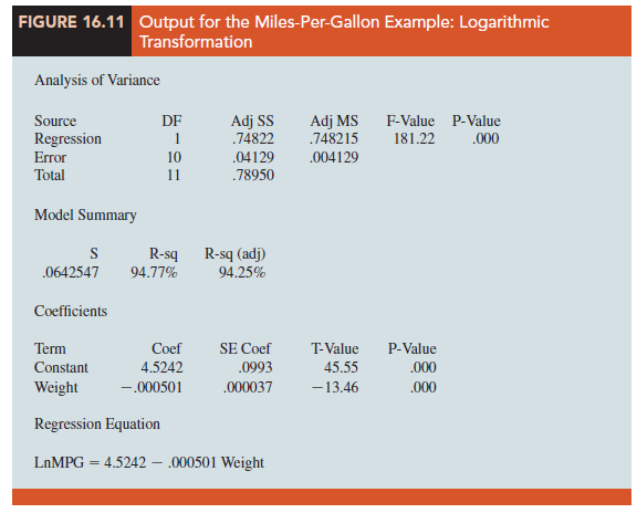
Often the problem of nonconstant variance can be corrected by transforming the dependent variable to a different scale. For instance, if we work with the logarithm of the dependent variable instead of the original dependent variable, the effect will be to compress the values of the dependent variable and thus diminish the effects of nonconstant variance. Most statistical packages provide the ability to apply logarithmic transformations using either the base 10 (common logarithm, log10) or the base e = 2.71828 (natural logarithm, ln). We applied a natural logarithmic transformation to the miles- per-gallon data and developed the estimated regression equation relating weight to the natural logarithm of miles-per-gallon. The regression results obtained by using the natural logarithm of miles-per-gallon as the dependent variable, labeled LnMPG in the output, are shown in Figure 16.11; Figure 16.12 is the corresponding standardized residual plot.
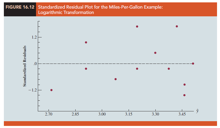
Looking at the residual plot in Figure 16.12, we see that the wedge-shaped pattern has now disappeared. Moreover, none of the observations is identified as having a large standardized residual. The model with the logarithm of miles per gallon as the dependent variable is statistically significant and provides an excellent fit to the observed data. Hence, we would recommend using the estimated regression equation
LnMPG = 4.5242 – .000501 Weight
To predict the miles-per-gallon rating for an automobile that weighs 2500 pounds, we first develop an estimate of the logarithm of the miles-per-gallon rating.
LnMPG = 4.5242 – .000501(2500) = 3.2717
The miles-per-gallon estimate is obtained by finding the number whose natural logarithm is 3.2717. Using a calculator with an exponential function, or raising e to the power 3.2717, we obtain 26.36 miles per gallon.
Another approach to problems of nonconstant variance is to use 1/y as the dependent variable instead of y. This type of transformation is called a reciprocal transformation. For instance, if the dependent variable is measured in miles per gallon, the reciprocal transformation would result in a new dependent variable whose units would be 1/(miles per gallon) or gallons per mile. In general, there is no way to determine whether a logarithmic transformation or a reciprocal transformation will perform better without actually trying each of them.
4. Nonlinear Models That Are Intrinsically Linear
Models in which the parameters (β0, β1, … , βp) have exponents other than 1 are called nonlinear models. However, for the case of the exponential model, we can perform a transformation of variables that will enable us to perform regression analysis with equation (16.1), the general linear model. The exponential model involves the following regression equation.
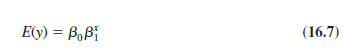
This regression equation is appropriate when the dependent variable y increases or decreases by a constant percentage, instead of by a fixed amount, as x increases.
As an example, suppose sales for a product y are related to advertising expenditure x (in thousands of dollars) according to the following regression equation.
![]()
Thus, for x = 1, E( y) = 500(1.2)1 = 600; for x = 2, E( y) = 500(1.2)2 = 720; and for x = 3, E( y) = 500(1.2)3 = 864. Note that E( y) is not increasing by a constant amount in this case, but by a constant percentage; the percentage increase is 20%.
We can transform this nonlinear regression equation to a linear regression equation by taking the natural logarithm of both sides of equation (16.7).
![]()
Now if we let y’ = ln E( y), β’0 = ln β0, and β’1 = ln β1, we can rewrite equation (16.8) as
![]()
It is clear that the formulas for simple linear regression can now be used to develop estimates of β’0 and β’1. Denoting the estimates as b’0 and b’1 leads to the following estimated regression equation.
To obtain predictions of the original dependent variable y given a value of x, we would first substitute the value of x into equation (16.9) to compute y’, and then raise e to the power of y’ to obtain the prediction of y, or the expected value of y, in its original units.
Many nonlinear models cannot be transformed into an equivalent linear model. However, such models have had limited use in business and economic applications. Furthermore, the mathematical background needed for study of such models is beyond the scope of this text.
Source: Anderson David R., Sweeney Dennis J., Williams Thomas A. (2019), Statistics for Business & Economics, Cengage Learning; 14th edition.
30 Aug 2021
31 Aug 2021
30 Aug 2021
30 Aug 2021
28 Aug 2021
30 Aug 2021