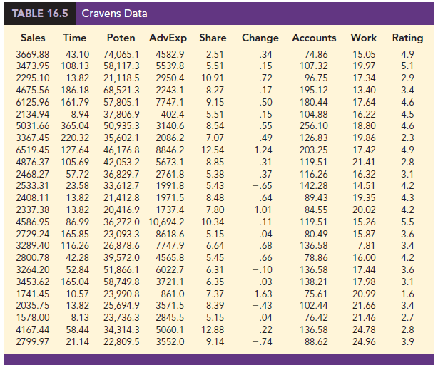
In introducing multiple regression analysis, we used the Butler Trucking example extensively. The small size of this problem was an advantage in exploring introductory concepts but would make it difficult to illustrate some of the variable selection issues involved in model building. To provide an illustration of the variable selection procedures discussed in the next section, we introduce a data set consisting of 25 observations on eight independent variables. Permission to use these data was provided by Dr. David W. Cravens of the Department of Marketing at Texas Christian University. Consequently, we refer to the data set as the Cravens data.1
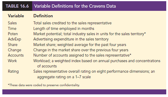
The Cravens data are for a company that sells products in several sales territories, each of which is assigned to a single sales representative. A regression analysis was conducted to determine whether a variety of predictor (independent) variables could explain sales in each territory. A random sample of 25 sales territories resulted in the data in Table 16.5; the variable definitions are given in Table 16.6.
As a preliminary step, let us consider the sample correlation coefficients between each pair of variables. Figure 16.13 is the correlation matrix obtained using statistical software. Note that the sample correlation coefficient between Sales and Time is .623, between Sales and Poten is .598, and so on.
Looking at the sample correlation coefficients between the independent variables, we see that the correlation between Time and Accounts is .758; hence, if Accounts were used as an independent variable, Time would not add much more explanatory power to the model. Recall the rule-of-thumb test from the discussion of multicollinearity in Section 15.4: Multicollinearity can cause problems if the absolute value of the sample correlation coefficient exceeds .7 for any two of the independent variables. If possible, then, we should avoid including both Time and Accounts in the same regression model. The sample correlation coefficient of .549 between Change and Rating is also high and may warrant further consideration.
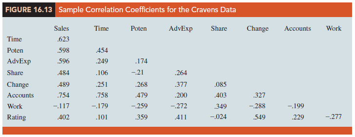
Looking at the sample correlation coefficients between Sales and each of the independent variables can give us a quick indication of which independent variables are, by themselves, good predictors. We see that the single best predictor of Sales is Accounts, because it has the highest sample correlation coefficient (.754). Recall that for the case of one independent variable, the square of the sample correlation coefficient is the coefficient of determination. Thus, Accounts can explain (.754)2(100), or 56.85%, of the variability in Sales. The next most important independent variables are Time, Poten, and AdvExp, each with a sample correlation coefficient of approximately .6.
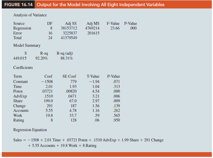
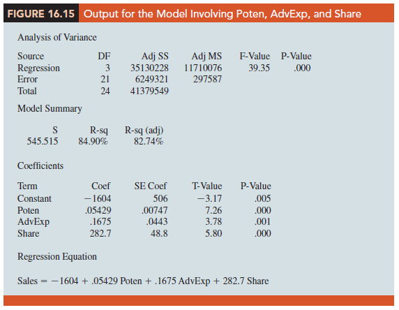
Although there are potential multicollinearity problems, let us consider developing an estimated regression equation using all eight independent variables. Using statistical software, we obtain the results in Figure 16.14. The eight-variable multiple regression model has an R-sq (adj) value of 88.31%. Note, however, that the p-values for the t tests of individual parameters show that only Poten, AdvExp, and Share are significant at the a = .05 level, given the effect of all the other variables. Hence, we might be inclined to investigate the results that would be obtained if we used just those three variables. Figure 16.15 shows the results obtained for the estimated regression equation with those three variables. We see that the estimated regression equation has an R-sq (adj) value of 82.74%, which, although not quite as good as that for the eight-independent-variable estimated regression equation, is high.
How can we find an estimated regression equation that will do the best job given the data available? One approach is to compute all possible regressions. That is, we could develop 8 one-variable estimated regression equations (each of which corresponds to one of the independent variables), 28 two-variable estimated regression equations (the number of combinations of eight variables taken two at a time), and so on. In all, for the Cravens data, 255 different estimated regression equations involving one or more independent variables would have to be fitted to the data.
With the powerful statistical software packages available today, it is possible to compute all possible regressions. But doing so involves a great amount of computation and requires the model builder to review a large volume of computer output, much of which is associated with obviously poor models. Statisticians prefer a more systematic approach to selecting the subset of independent variables that provide the best estimated regression equation. In the next section, we introduce some of the more popular approaches.
Source: Anderson David R., Sweeney Dennis J., Williams Thomas A. (2019), Statistics for Business & Economics, Cengage Learning; 14th edition.
30 Aug 2021
31 Aug 2021
30 Aug 2021
30 Aug 2021
31 Aug 2021
28 Aug 2021