Developing Discrete Probability Distributions

The probability distribution for a random variable describes how probabilities are distributed over the values of the random variable. For a discrete random variable x, a probability function, denoted by f(x), provides the probability for each value of the random variable. The classical, subjective, and relative frequency methods of assign­ing probabilities can be used to develop discrete probability distributions. Application of this methodology leads to what we call tabular discrete probability distributions; that is, probability distributions that are presented in a table.

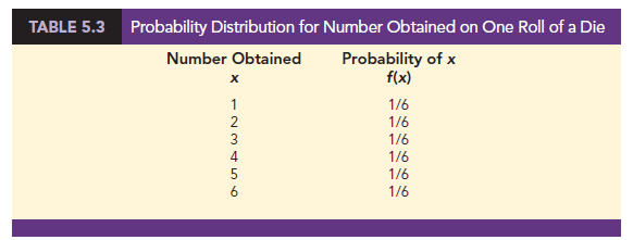
The classical method of assigning probabilities to values of a random variable is applicable when the experimental outcomes generate values of the random variable that are equally likely. For instance, consider the experiment of rolling a die and observing the number on the upward face. It must be one of the numbers 1, 2, 3, 4, 5, or 6 and each of these outcomes is equally likely. Thus, if we let x = number obtained on one roll of a die and f(x) = the probability of x, the probability distribution of x is given in Table 5.3.

The subjective method of assigning probabilities can also lead to a table of values of the random variable together with the associated probabilities. With the subjective method the individual developing the probability distribution uses their best judg­ment to assign each probability. So, unlike probability distributions developed using the classical method, different people can be expected to obtain different probability distributions.

The relative frequency method of assigning probabilities to values of a random variable is applicable when reasonably large amounts of data are available. We then treat the data as if they were the population and use the relative frequency method to assign probabilities to the experimental outcomes. The use of the relative frequency method to develop discrete probability distributions leads to what is called an empirical discrete distribution. With the large amounts of data available today (e.g., scanner data, credit card data), this type of probability distribution is becoming more widely used in practice. Let us illustrate by considering the sale of automobiles at a dealership.

We will use the relative frequency method to develop a probability distribution for the number of cars sold per day at DiCarlo Motors in Saratoga, New York. Over the past 300 days, DiCarlo has experienced 54 days with no automobiles sold, 117 days with 1 automobile sold, 72 days with 2 automobiles sold, 42 days with 3 automobiles sold, 12 days with 4 automobiles sold, and 3 days with 5 automobiles sold. Suppose we consider the experiment of observing a day of operations at DiCarlo Motors and define the random variable of interest as x = the number of automobiles sold during a day. Using the relative frequencies to assign probabilities to the values of the random variable x, we can develop the probability distribution for x.

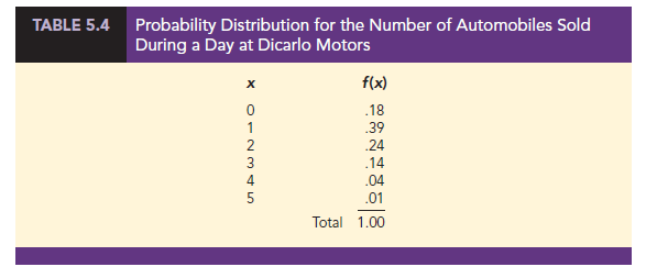
In probability function notation, f (0) provides the probability of 0 automobiles sold, f(1) provides the probability of 1 automobile sold, and so on. Because historical data show 54 of 300 days with 0 automobiles sold, we assign the relative frequency 54/300 = .18 to f (0), indicating that the probability of 0 automobiles being sold during a day is .18. Similarly, because 117 of 300 days had 1 automobile sold, we assign the relative frequency 117/300 = .39 to f(1), indicating that the probability of exactly 1 automobile being sold during a day is .39. Continuing in this way for the other values of the random variable, we compute the values for f (2), f(3), f(4), and f(5) as shown in Table 5.4.

A primary advantage of defining a random variable and its probability distribution is that once the probability distribution is known, it is relatively easy to determine the probab­ility of a variety of events that may be of interest to a decision maker. For example, using the probability distribution for DiCarlo Motors as shown in Table 5.4, we see that the most probable number of automobiles sold during a day is 1 with a probability of f(1) = .39. In addition, there is an f(3) + f(4) + f(5) = .14 + .04 + .01 = .19 probability of selling 3 or more automobiles during a day. These probabilities, plus others the decision maker may ask about, provide information that can help the decision maker understand the process of selling automobiles at DiCarlo Motors.

In the development of a probability function for any discrete random variable, the fol­lowing two conditions must be satisfied.

Table 5.4 shows that the probabilities for the random variable x satisfy equation (5.1); f(x) is greater than or equal to 0 for all values of x. In addition, because the probabilities sum to 1, equation (5.2) is satisfied. Thus, the DiCarlo Motors probability function is a valid discrete probability function.

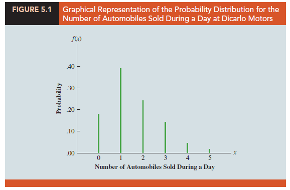
We can also show the DiCarlo Motors probability distribution graphically. In Figure 5.1 the values of the random variable x for DiCarlo Motors are shown on the horizontal axis and the probability associated with these values is shown on the vertical axis.

In addition to the probability distributions shown in tables, a formula that gives the probability function, f(x), for every value of x is often used to describe probability distri­butions. The simplest example of a discrete probability distribution given by a formula is the discrete uniform probability distribution. Its probability function is defined by equation (5.3).

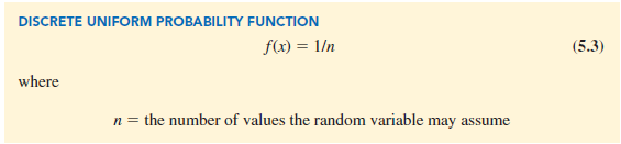
For example, consider again the experiment of rolling a die. We define the random variable x to be the number of dots on the upward face. For this experiment, n = 6 values are possible for the random variable; x = 1, 2, 3, 4, 5, 6. We showed earlier how the probability distribution for this experiment can be expressed as a table. Since the probab­ilities are equally likely, the discrete uniform probability function can also be used. The probability function for this discrete uniform random variable is

f (x) = 1/6     x = 1, 2, 3, 4, 5, 6

Several widely used discrete probability distributions are specified by formulas. Three important cases are the binomial, Poisson, and hypergeometric distributions; these distribu­tions are discussed later in the chapter.

Source:  Anderson David R., Sweeney Dennis J., Williams Thomas A. (2019), Statistics for Business & Economics, Cengage Learning; 14th edition.