Time Series Patterns

A time series is a sequence of observations on a variable measured at successive points in time or over successive periods of time. The measurements may be taken every hour, day, week, month, or year, or at any other regular interval.^[1] The pattern of the data is an important factor in understanding how the time series has behaved in the past. If such be­havior can be expected to continue in the future, we can use the past pattern to guide us in selecting an appropriate forecasting method.

To identify the underlying pattern in the data, a useful first step is to construct a time series plot. A time series plot is a graphical presentation of the relationship between time and the time series variable; time is on the horizontal axis and the time series values are shown on the vertical axis. Let us review some of the common types of data patterns that can be identified when examining a time series plot.

1. Horizontal Pattern

A horizontal pattern exists when the data fluctuate around a constant mean. To illustrate a time series with a horizontal pattern, consider the 12 weeks of data in Table 17.1.

These data show the number of gallons of gasoline sold by a gasoline distributor in Bennington, Vermont, over the past 12 weeks. The average value or mean for this time series is 19.25 or 19,250 gallons per week. Figure 17.1 shows a time series plot for these data. Note how the data fluctuate around the sample mean of 19,250 gallons. Although random variability is present, we would say that these data follow a horizontal pattern.

The term stationary time series² is used to denote a time series whose statistical properties are independent of time. In particular this means that

1. The process generating the data has a constant mean.
2. The variability of the time series is constant over time.

A time series plot for a stationary time series will always exhibit a horizontal pattern. But simply observing a horizontal pattern is not sufficient evidence to conclude that the time series is stationary. More advanced texts on forecasting discuss procedures for determining if a time series is stationary and provide methods for transforming a time series that is not stationary into a stationary series.

Changes in business conditions can often result in a time series that has a horizontal pattern shifting to a new level. For instance, suppose the gasoline distributor signs a contract with the Vermont State Police to provide gasoline for state police cars located in southern Vermont. With this new contract, the distributor expects to see a major increase in weekly sales starting in week 13. Table 17.2 shows the number of gallons of gasoline sold for the original time series and for the 10 weeks after signing the new contract. Fig­ure 17.2 shows the corresponding time series plot. Note the increased level of the time series beginning in week 13. This change in the level of the time series makes it more difficult to choose an appropriate forecasting method. Selecting a forecasting method that adapts well to changes in the level of a time series is an important consideration in many practical applications.

2. Trend Pattern

Although time series data generally exhibit random fluctuations, a time series may also show gradual shifts or movements to relatively higher or lower values over a longer period of time. If a time series plot exhibits this type of behavior, we say that a trend pattern exists. A trend is usually the result of long-term factors such as population increases or decreases, changing demographic characteristics of the population, technology, and/or consumer preferences.

To illustrate a time series with a trend pattern, consider the time series of bicycle sales for a particular manufacturer over the past 10 years, as shown in Table 17.3 and Figure 17.3. Note that 21,600 bicycles were sold in year one, 22,900 were sold in year two, and so on. In year 10, the most recent year, 31,400 bicycles were sold. Visual inspection of the time series plot shows some up and down movement over the past 10 years, but the time series also seems to have a systematically increasing or upward trend.

The trend for the bicycle sales time series appears to be linear and increasing over time, but sometimes a trend can be described better by other types of patterns. For instance, the data in Table 17.4 and the corresponding time series plot in Figure 17.4 show the sales for a cholesterol drug since the company won FDA approval for it 10 years ago. The time series increases in a nonlinear fashion; that is, the rate of change of revenue does not increase by a constant amount from one year to the next. In fact, the revenue appears to be growing in an exponential fashion. Exponential relationships such as this are appropriate when the percentage change from one period to the next is relatively constant.

3. Seasonal Pattern

The trend of a time series can be identified by analyzing multiyear movements in historical data. Seasonal patterns are recognized by seeing the same repeating patterns over succes­sive periods of time. For example, a manufacturer of swimming pools expects low sales activity in the fall and winter months, with peak sales in the spring and summer months. Manufacturers of snow removal equipment and heavy clothing, however, expect just the opposite yearly pattern. Not surprisingly, the pattern for a time series plot that exhibits a repeating pattern over a one-year period due to seasonal influences is called a seasonal pattern. While we generally think of seasonal movement in a time series as occurring within one year, time series data can also exhibit seasonal patterns of less than one year in duration. For example, daily traffic volume shows within-the-day “seasonal” behavior, with peak levels occurring during rush hours, moderate flow during the rest of the day and early evening, and light flow from midnight to early morning.

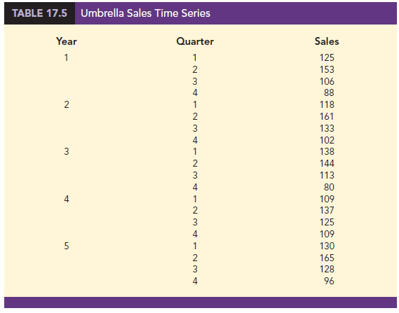
As an example of a seasonal pattern, consider the number of umbrellas sold at a clothing store over the past five years. Table 17.5 shows the time series and Figure 17.5 shows the corresponding time series plot. The time series plot does not indicate any long-term trend in sales. In fact, unless you look carefully at the data, you might conclude that the data follow a horizontal pattern. But closer inspection of the time series plot reveals a regular pattern in the data. That is, the first and third quarters have moderate sales, the second quarter has the highest sales, and the fourth quarter tends to have the lowest sales volume. Thus, we would conclude that a quarterly seasonal pattern is present.

4. Trend and Seasonal Pattern

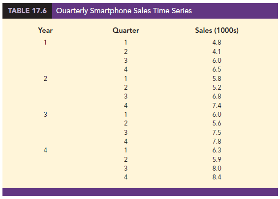
Some time series include a combination of a trend and seasonal pattern. For instance, the data in Table 17.6 and the corresponding time series plot in Figure 17.6 show smartphone sales for a particular manufacturer over the past four years. Clearly, an increasing trend is present. But, Figure 17.6 also indicates that sales are lowest in the second quarter of each year and increase in quarters 3 and 4. Thus, we conclude that a seasonal pattern also exists for smartphone sales. In such cases we need to use a forecasting method that has the capa­bility to deal with both trend and seasonality.

5. Cyclical Pattern

A cyclical pattern exists if the time series plot shows an alternating sequence of points below and above the trend line lasting more than one year. Many economic time series exhibit cyclical behavior with regular runs of observations below and above the trend line.

Often, the cyclical component of a time series is due to multiyear business cycles. For ex­ample, periods of moderate inflation followed by periods of rapid inflation can lead to time series that alternate below and above a generally increasing trend line (e.g., a time series for housing costs). Business cycles are extremely difficult, if not impossible, to forecast. As a result, cyclical effects are often combined with long-term trend effects and referred to as trend-cycle effects. In this chapter we do not deal with cyclical effects that may be present in the time series.

6. Selecting a Forecasting Method

The underlying pattern in the time series is an important factor in selecting a forecasting method. Thus, a time series plot should be one of the first things developed when trying to determine which forecasting method to use. If we see a horizontal pattern, then we need to select a method appropriate for this type of pattern. Similarly, if we observe a trend in the data, then we need to use a forecasting method that has the capability to handle trend effectively. The next two sections illustrate methods that can be used in situations where the underlying pattern is horizontal; in other words, no trend or seasonal effects are present. We then consider methods appropriate when trend and/or seasonality are present in the data.

Source:  Anderson David R., Sweeney Dennis J., Williams Thomas A. (2019), Statistics for Business & Economics, Cengage Learning; 14th edition.