Inventory Control or Management in Production and Operation Management

1. Meaning of Inventory

Inventory generally refers to the materials in stock. It is also called the idle resource of an enterprise. Inventories represent those items which are either stocked for sale or they are in the process of manufacturing or they are in the form of materials, which are yet to be utilised. The interval between receiving the purchased parts and transforming them into final products varies from industries to industries depending upon the cycle time of manufacture. It is, therefore, necessary to hold inventories of various kinds to act as a buffer between supply and demand for efficient operation of the system. Thus, an effective control on inventory is a must for smooth and efficient running of the production cycle with least interruptions.

2. Reasons for Keeping Inventories

1. To stabilise production: The demand for an item fluctuates because of the number of factors, g., seasonality, production schedule etc. The inventories (raw materials and components) should be made available to the production as per the demand failing which results in stock out and the production stoppage takes place for want of materials. Hence, the inventory is kept to take care of this fluctuation so that the production is smooth.
2. To take advantage of price discounts: Usually the manufacturers offer discount for bulk buying and to gain this price advantage the materials are bought in bulk even though it is not required immediately. Thus, inventory is maintained to gain economy in purchasing.
3. To meet the demand during the replenishment period: The lead time for procurement of materials depends upon many factors like location of the source, demand supply condition, etc. So inventory is maintained to meet the demand during the procurement (replenishment) period.
4. To prevent loss of orders (sales): In this competitive scenario, one has to meet the delivery schedules at 100 per cent service level, means they cannot afford to miss the delivery schedule which may result in loss of sales. To avoid the organizations have to maintain inventory.
5. To keep pace with changing market conditions: The organizations have to anticipate the changing market sentiments and they have to stock materials in anticipation of non-availability of materials or sudden increase in prices.
6. Sometimes the organizations have to stock materials due to other reasons like suppliers minimum quantity condition, seasonal availability of materials or sudden increase in prices.

3. Meaning of Inventory Control

Inventory control is a planned approach of determining what to order, when to order and how much to order and how much to stock so that costs associated with buying and storing are optimal without interrupting production and sales. Inventory control basically deals with two problems: (i) When should an order be placed? (Order level), and (ii) How much should be ordered? (Order quantity).

These questions are answered by the use of inventory models. The scientific inventory control system strikes the balance between the loss due to non-availability of an item and cost of carrying the stock of an item. Scientific inventory control aims at maintaining optimum level of stock of goods required by the company at minimum cost to the company.

4. Objectives of Inventory Control

1. To ensure adequate supply of products to customer and avoid shortages as far as possible.
2. To make sure that the financial investment in inventories is minimum (i.e., to see that the working capital is blocked to the minimum possible extent).
3. Efficient purchasing, storing, consumption and accounting for materials is an important objective.
4. To maintain timely record of inventories of all the items and to maintain the stock within the desired limits.
5. To ensure timely action for replenishment.
6. To provide a reserve stock for variations in lead times of delivery of materials.
7. To provide a scientific base for both short-term and long-term planning of materials.

5. Benefits of Inventory Control

It is an established fact that through the practice of scientific inventory control, following are the benefits of inventory control:

1. Improvement in customer’s relationship because of the timely delivery of goods and service.
2. Smooth and uninterrupted production and, hence, no stock out.
3. Efficient utilisation of working capital. Helps in minimising loss due to deterioration, obsolescence damage and pilferage.
4. Economy in purchasing.
5. Eliminates the possibility of duplicate ordering.

6. Techniques of Inventory Control

In any organization, depending on the type of business, inventory is maintained. When the number of items in inventory is large and then large amount of money is needed to create such inventory, it becomes the concern of the management to have a proper control over its ordering, procurement, maintenance and consumption. The control can be for order quality and order frequency.

The different techniques of inventory control are: (1) ABC analysis, (2) HML analysis, (3) VED analysis, (4) FSN analysis, (5) SDE analysis, (6) GOLF analysis and (7) SOS analysis. The most widely used method of inventory control is known as ABC analysis. In this technique, the total inventory is categorised into three sub-heads and then proper exercise is exercised for each sub-heads.

1. ABC analysis: In this analysis, the classification of existing inventory is based on annual consumption and the annual value of the items. Hence we obtain the quantity of inventory item consumed during the year and multiply it by unit cost to obtain annual usage cost. The items are then arranged in the descending order of such annual usage cost. The analysis is carried out by drawing a graph based on the cumulative number of items and cumulative usage of consumption cost. Classification is done as follows:

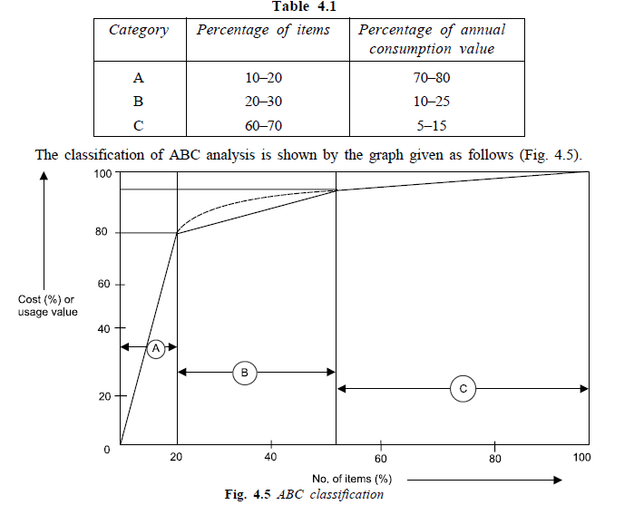
Once ABC classification has been achieved, the policy control can be formulated as follows:

A-Item: Very tight control, the items being of high value. The control need be exercised at higher level of authority.

B-Item: Moderate control, the items being of moderate value. The control need be exercised at middle level of authority.

C-Item: The items being of low value, the control can be exercised at gross root level of authority, i.e., by respective user department managers.

2. HML analysis: In this analysis, the classification of existing inventory is based on unit price of the items. They are classified as high price, medium price and low cost items.
3. VED analysis: In this analysis, the classification of existing inventory is based on criticality of the items. They are classified as vital, essential and desirable items. It is mainly used in spare parts inventory.
4. FSN analysis: In this analysis, the classification of existing inventory is based consumption of the items. They are classified as fast moving, slow moving and non-moving items.
5. SDE analysis: In this analysis, the classification of existing inventory is based on the items.
6. GOLF analysis: In this analysis, the classification of existing inventory is based sources of the items. They are classified as Government supply, ordinarily available, local availability and foreign source of supply items.
7. SOS analysis: In this analysis, the classification of existing inventory is based nature of supply of items. They are classified as seasonal and off-seasonal items.

For effective inventory control, combination of the techniques of ABC with VED or ABC with HML or VED with HML analysis is practically used.

7. Inventory Model

Economic Order Quantity (EOQ)

Inventory models deal with idle resources like men, machines, money and materials. These models are concerned with two decisions: how much to order (purchase or produce) and when to order so as to minimize the total cost.

For the first decision—how much to order, there are two basic costs are considered namely, inventory carrying costs and the ordering or acquisition costs. As the quantity ordered is increased, the inventory carrying cost increases while the ordering cost decreases. The ‘order quantity’ means the quantity produced or procured during one production cycle. Economic order quantity is calculated by balancing the two costs. Economic Order Quantity (EOQ) is that size of order which minimizes total costs of carrying and cost of ordering.

1. , Minimum Total Cost occurs when Inventory Carrying Cost = Ordering Cost

Economic order quantity can be determined by two methods:

1. Tabulation method.
2. Algebraic method.

7.1. Determination of EOQ by Tabulation (Trial & Error) Method

This method involves the following steps:

1. Select the number of possible lot sizes to purchase.
2. Determine average inventory carrying cost for the lot purchased.
3. Determine the total ordering cost for the orders placed.
4. Determine the total cost for each lot size chosen which is the summation of inventory carrying cost and ordering cost.
5. Select the ordering quantity, which minimizes the total cost.

The data calculated in a tabular column can plotted showing the nature of total cost, inventory cost and ordering cost curve against the quantity ordered as in Fig. 4.6.

ILLUSTRATION 3: The XYZ Ltd. carries a wide assortment of items for its customers. One of its popular items has annual demand of 8000 units. Ordering cost per order is found to be Rs. 12.5. The carrying cost of average inventory is 20% per year and the cost per unit is Re. 1.00. Determine the optimal economic quantity and make your recommendations.

SOLUTION:

The table and the graph indicates that an order size of 1000 units will gives the lowest total cost among the different alternatives. It also shows that minimum total cost occurs when carrying cost is equal to ordering cost.

7.2. Determination of EOQ by Analytical Method

In order to derive an economic lot size formula following assumptions are made:

1. Demand is known and uniform.
2. Let D denotes the total number of units purchase/produced and Q denotes the lot size in each production run.
3. Shortages are not permitted, e., as soon as the level of the inventory reaches zero, the inventory is replenished.
4. Production or supply of commodity is instantaneous.
5. Lead-time is zero.
6. Set-up cost per production run or procurement cost is C₃.
7. Inventory carrying cost is C₁ = CI, where C is the unit cost and I is called inventory carrying cost expressed as a percentage of the value of the average inventory.

This fundamental situation can be shown on an inventory-time diagram, (Fig. 4.7) with Q on the vertical axis and the time on the horizontal axis. The total time period (one year) is divided into n parts.

The most economic point in terms of total inventory cost exists where,

Inventory carrying cost = Annual ordering cost (set-up cost)

Average inventory = 1/2 (maximum level + minimum level)

                              = (Q + 0)/2 = Q/2

Total inventory carrying cost   =    Average inventory x Inventory carrying cost per unit

Total inventory carrying cost =            Q/2 x C_x = QC_x/2                                     …(1)

Total annual ordering costs   =   Number of orders per year       x   Ordering         cost per order

Total annual ordering costs =            (D/Q) x C₃ = (D/Q)C₃                                   ..(2)

Now, summing up the total inventory cost and the total ordering cost, we get the total inventory cost C(Q).

Total cost of production run = Total inventory carrying cost + Total annual ordering costs

C(Q) = QC₁/2 + (D/Q)C₃         (cost equation)                . (3)

But, the total cost is minimum when the inventory carrying costs becomes equal to the total annual ordering costs. Therefore,

ILLUSTRATION 4: An oil engine manufacturer purchases lubricants at the rate of Rs. 42 per piece from a vendor. The requirements of these lubricants are 1800 per year. What should be the ordering quantity per order, if the cost per placement of an order is Rs. 16 and inventory carrying charges per rupee per year is 20 paise.

SOLUTION: Given data are:

Number of lubricants to be purchased, D = 1800 per year

Procurement cost, C₃ = Rs. 16 per order

Inventory carrying cost, CI = C_x = Rs. 42 x Re. 0.20 = Rs. 8.40 per year

Then, optimal quantity (EOQ),

ILLUSTRATION 5: A manufacturing company purchase 9000 parts of a machine for its annual requirements ordering for month usage at a time, each part costs Rs. 20. The ordering cost per order is Rs. 15 and carrying charges are 15% of the average inventory per year. You have been assigned to suggest a more economical purchase policy for the company. What advice you offer and how much would it save the company per year?

SOLUTION: Given data are:

Number of lubricants to be purchased, D = 9000 parts per year

Cost of part, Cs = Rs. 20

Procurement cost, C3 = Rs. 15 per order

Inventory carrying cost, CI = C1 = 15% of average inventory per year

= Rs. 20 × 0.15 = Rs. 3 per each part per year

Then, optimal quantity (EOQ),

and Optimum order interval,

If the company follows the policy of ordering every month, then the annual ordering cost is

= Rs 12 × 15 = Rs. 180

Lot size of inventory each month = 9000/12 = 750

Average inventory at any time = Q/2 = 750/2 = 375

Therefore,storage cost at any time = 375 × C1 = 375 × 3 = Rs. 1125

Total annual cost = 1125 + 180 = Rs. 1305

Hence, the company should purchase 300 parts at time interval of 1/30 year instead of ordering 750 parts each month. The net saving of the company will be

= Rs. 1305 – Rs. 900 = Rs. 405 per year.

Source: KumarAnil, Suresh N. (2009), Production and operations management, New Age International Pvt Ltd; 2nd Ed. edition.