Data Analysis Using STATA: Use and Interpretation

Stata is a general-purpose statistical software package created in 1985 by StataCorp. The name Stata is a syllabic abbreviation of the words statistics and data. The FAQ for the official forum of Stata insists that the correct English pronunciation of Stata “must remain a mystery”; any of “Stay-ta”, “Sta-ta” or “Stah-ta” (rhymes of the three pronunciations of ‘data’) are considered acceptable. More recent updates indicate

How to Install and Activate Stata on a Windows Computer

In this post, we will show you how to install and activate Stata, that is a software allowing you to store and manage data, undertake statistical analysis on your data, and create some really nice graphs. Most of its users work in research, especially in the fields of economics, sociology, political science, biomedicine and

How to Install and Activate Stata on a Mac Computer

Step 1: Download Stata 1. Go to http://download.stata.com/download. The following login box should appear in your browser. Enter your username and password (as provided in the email from Survey Design and Analysis), as well as the other information requested, and click ‘Log in’: 2. Select the ‘Mac’ option for your operating system: 3. Then

Quick Overview of Stata User Interface

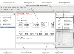
Stata’s capabilities include data management, statistical analysis, graphics, simulations, regression, and custom programming. It also has a system to disseminate user-written programs that lets it grow continuously. This article introduces the core of Stata’s interface: its main windows, its toolbar, its menus, and its dialogs. 1. The windows The five main windows are the History,

3 Comments

Using the Stata Viewer

The Viewer’s purpose The Viewer is a versatile tool in Stata. It will be the first place you can turn for help within Stata, but it is far more than just a help system. You can also use the Viewer to add, delete, and manage third-party extensions to Stata that are known as community-contributed

Getting help in Stata

Stata’s help system provides a wealth of information to help you learn and use Stata. To find out which Stata command will perform the statistical or data management task you would like to do, you should generally follow these

1 Comments

Finding and Installing New Commands or User-Written Programs in Stata

Stata has a system to disseminate user-written programs that lets it grow continuously. So actually, there are a tremendous number of user-written programs for Stata available which, once installed, act just like official Stata commands. This article will show you how to find, install and update new commands or user-written programs in Stata. Finding

1 Comments

Opening and saving Stata datasets

Opening and saving datasets in Stata works similarly to those tasks in other computer applications. There are a few differences, however. First, it is possible to save and open files from within Stata’s Command window. Second, Stata allows just one dataset to be active at any one time. That is, while it is possible

1 Comments

Using the Data Editor in Stata

1. The Data Editor The Data Editor gives a spreadsheet-like view of data that are currently in memory. You can use it to enter new data, edit existing data, search through the dataset, and edit attributes of the data in the dataset, such as variable names, labels, and display formats, as well as value

1 Comments

Using the Variables Manager in Stata

1. The Variables Manager This chapter discusses Stata’s Variables Manager. To get started, open the automobile dataset by typing sysuse auto, clear in the Command window. You open the Variables Manager by selecting Data > Variables Manager or clicking on the Variables Manager button . The Variables Manager is a tool for managing properties

1 Comments

Importing data in Stata

One of the easiest ways to get data into Stata is often overlooked: you can copy data from most applications that understand the concept of a table and then paste the data into the Data Editor. Copying and pasting is a great way to bring data into Stata, but if you need a clear audit trail for your data, you will need another way to bring data into Stata. The rest of this chapter will explain how to do this. You will also learn methods that lend themselves better to repetitive tasks and methods for importing data from a wide

Labeling data in Stata

1. Making data readable This chapter discusses, in brief, labeling of the dataset, variables, and values. Such labeling is critical to careful use of data. Labeling variables with descriptive names clarifies their meanings. Labeling values of numerical categorical variables ensures that the real-world meanings of the encodings are not forgotten. These points are crucial

Listing data and basic command syntax in Stata

1. Command syntax This chapter gives a basic lesson on Stata’s command syntax while showing how to control the appearance of a data list. As we have seen throughout this manual, you have a choice between using menus and dialogs and using the Command window. Although many find the menus more natural and the

Creating new variables in Stata

1. Generate and replace This chapter shows the basics of creating and modifying variables in Stata. We saw how to work with the Data Editor in [GSW] 6 Using the Data Editor—this chapter shows how we would do this from the Command window. The two primary commands used for this are generate for creating

Deleting variables and observations in Stata

1. Clear, drop, and keep In this chapter, we will present the tools for paring observations and variables from a dataset. We saw how to do this using the Data Editor in [GSW] 6 Using the Data Editor; this chapter presents the methods for doing so from the Command window. There are three main

Using the Do-file Editor—automating Stata

1. The Do-file Editor Stata comes with an integrated text editor called the Do-file Editor, which can be used for many tasks. It gets its name from the term do-file, which is a file containing a list of commands for Stata to run (called a batch file or a script in other settings). See

Graphing data in Stata

1. Working with graphs Stata has a rich system for graphical representation of data. The main command for creating graphs is unsurprisingly named graph. Behind this plain name is a wealth of tools. In this chapter, we will make one simple graph to point out the basics of the Graph window. See the [G]

Editing graphs in Stata

1. The Graph Editor With Stata’s Graph Editor, you can change almost anything on your graph; you can add text, lines, arrows, and markers wherever you like. We will first make a graph to edit and will then point out the tools in the Graph Editor. Start by opening the automobile dataset: sysuse auto.

Saving and printing results by using logs in Stata

1. Using logs in Stata When you work on an analysis, it is worthwhile to behave like a bench scientist and keep a lab notebook of your actions so that your work can be easily replicated. Everyone has a feeling of complete omniscience while working intensely—this feeling is wonderful but fleeting. The next day,

1 Comments

Setting font and window preferences in Stata

1. Changing and saving fonts and sizes and positions of your windows You may find that you would like to change the fonts and display style of Stata’s windows, depending on your monitor resolution and personal preferences. At the same time, there could be requirements for font usage, say, when you submit graphs to