There are two steps in this method: (1) high-ranking executives estimate probable sales, and (2) an average estimate is calculated. The assumption is that the executives are well informed about the industry outlook and the company’s market position, capabilities, and marketing program. All should support their estimates with factual material and explain their rationales.
Companies using the jury of executive opinion method do so for one or more of four reasons:
- This is a quick and easy way to turn out a forecast.
- This is a way to pool the experience and judgment of well-informed people.
- This may be the only feasible approach if the company is so young that it has not yet accumulated the experience to use other forecasting methods.
- This method may be used when adequate sales and market statistics are missing, or when these figures have not yet been put into the format required for more sophisticated forecasting methods.
The jury of executive opinion method has weaknesses. Its findings are based primarily on opinion, and factual evidence to support the forecast is often sketchy. This approach adds to the work load of key executives, requiring them to spend time that they would otherwise devote to their areas of main responsibility. And a forecast made by this method is difficult to break down into estimates of probable sales by products, by time intervals, by markets, by customers, and so on.
1. Poll of Sales Force Opinion
In the poll of sales force opinion method, often tagged “the grass-roots approach,” individual sales personnel forecast sales for their territories; then individual forecasts are combined and modified, as management thinks necessary, to form the company sales forecast. This approach appeals to practical sales managers because forecasting responsibility is assigned to those who produce the results. Furthermore, there is merit in utilizing the specialized knowledge of those in closest touch with market conditions. Because the salespeople help to develop the forecast, they should have greater confidence in quotas based upon it. Another attractive feature is that forecasts developed by this method are easy to break down according to products, territories, customers, intermediaries, and sales force.
But the poll of sales force opinion approach has weaknesses. Not generally trained to do forecasting, and influenced by current business conditions in their territories, salespersons tend to be overly optimistic or overly pessimistic about sales prospects. They are too near the trees to see the forest—they are often unaware of broad changes taking place in the economy and of trends in business conditions outside their own territories. Furthermore, if the “forecasts” of the sales staff are used in setting quotas, some sales personnel deliberately underestimate so that quotas are reached more easily.
To some extent, the weaknesses of this method can be overcome through training the sales force in forecasting techniques, by orienting them to factors influencing company sales, and by adjusting for consistent biases in individual salespersons’ forecasts. For most companies, however, implementing corrective actions is an endless task, because sales personnel turnover is constantly going on, and new staff members (whose biases are unknown at the start) submit their forecasts along with those of veteran sales personnel with known biases. In short, this method is based to such a large extent on judgment that it is not appropriate for most companies to use it as the only forecasting method. The poll of sales force opinion serves best as a method of getting an alternative estimate for use as a check on a sales forecast obtained through some other approach.
2. Projection of Past Sales
The projection of past sales method of sales forecasting takes a variety of forms. The simplest is to set the sales forecast for the coming year at the same figure as the current year’s actual sales, or the forecast may be made by adding a set percentage to last year’s sales, or to a moving average of the sales figures for several past years. For instance, if it is assumed that there will be the same percentage sales increase next year as this year, the forecaster might utilize a naive model projection such as

This year’s sales are inevitably related to last year’s. Similarly, next year’s sales are related to this year’s and to those of all preceding years. Projecting present sales levels is a simple and inexpensive forecasting method and may be appropriate for companies in more or less stable or “mature” industries—it is rare in such industries for a company’s sales to vary more than 15 percent plus or minus from the preceding year.
Time-series analysis. Not greatly different in principle from the simple projection of past sales is time-series analysis, a statistical procedure for studying historical sales data. This procedure involves isolating and measuring four chief types of sales variations: long-term trends, cyclical changes, seasonal variations, and irregular fluctuations. Then a mathematical model describing the past behavior of the series is selected, assumed values for each type of sales variation are inserted, and the sales forecast is “cranked out.”
For most companies, time-series analysis finds practical application mainly in making long-range forecasts. Predictions on a year-to-year basis, such as are necessary for an operating sales forecast, generally are little more than approximations. Only where sales patterns are clearly defined and relatively stable from year to year is time-series analysis appropriately used for short-term operating sales forecasts.
One drawback of time-series analysis is that it is difficult to “call the turns.” Trend and cycle analysis helps in explaining why a trend, once under way, continues, but predicting the turns often is more important. When turns for the better are called correctly, management can capitalize upon sales opportunities; when turns for the worst are called correctly, management can cut losses.
Exponential smoothing. One statistical technique for short-range sales forecasting, exponential smoothing, is a type of moving average that represents a weighted sum of all past numbers in a time series, with the heaviest weight placed on the most recent data.1 To illustrate, consider this simple but widely used form of exponential smoothing—a weighted average of this year’s sales is combined with the forecast of this year’s sales to arrive at the forecast for next year’s sales. The forecasting equation, in other words, is

The a in the equation is called the “smoothing constant” and is set between 0.0 and 1.0. If, for example, actual sales for this year came to 320 units of product, the sales forecast for this year was 350 units, and the smoothing constant was 0.3, the forecast for next year’s sales is
(0.30)(320) 4 – (0.7)(350) = 341 units of products
Determining the value of a is the main problem. If the series of sales data changes slowly, a should be small to retain the effect of earlier observations. If the series changes rapidly, a should be large so that the forecasts respond to these changes. In practice, a is estimated by trying several values and making retrospective tests of the associated forecast error. The a value leading to the smallest forecast error is then chosen for future smoothing.[1]
Evaluation of past sales projection methods. The key limitation of all past sales projection methods lies in the assumption that past sales history is the sole factor influencing future sales. No allowance is made for significant changes made by the company in its marketing program or by its competitors in theirs. Nor is allowance made for sharp and rapid upswings or downturns in business activity, nor is it usual to correct for poor sales performance extending over previous periods.
The accuracy of the forecast arrived at through projecting past sales depends largely upon how close the company is to the market saturation point. If the market is nearly 100 percent saturated, some argue that it is defensible to predict sales by applying a certain percentage figure to “cumulative past sales of the product still in the hands of users” to determine annual replacement demand. However, most often the company whose product has achieved nearly 100 percent market saturation finds, since most companies of this sort market durables or semidurables, that its prospective customers can postpone or accelerate their purchases to a considerable degree.
Past sales projection methods are most appropriately used for obtaining “check” forecasts against which forecasts secured through other means are compared. Most companies make some use of past sales projections in their sales forecasting procedures. The availability of numerous computer programs for time-series analysis and exponential smoothing has accelerated this practice.
3. Survey of Customers’ Buying Plans
What more sensible way to forecast than to ask customers about their future buying plans? Industrial marketers use this approach more than consumer-goods marketers, because it is easiest to use where the potential market consists of small numbers of customers and prospects, substantial sales are made to individual accounts, the manufacturer sells direct to users, and customers are concentrated in a few geographical areas (all more typical of industrial than consumer marketing). In such instances, it is relatively inexpensive to survey a sample of customers and prospects to obtain their estimated requirements for the product, and to project the results to obtain a sales forecast. Survey results, however, need tempering by management’s specialized knowledge and by contemplated changes in marketing programs. Few companies base forecasts exclusively on a survey of customers’ buying plans. The main reason lies in the inherent assumptions that customers know what they are going to do and that buyers’ plans, once made, will not change.
Even though the survey of customers’ buying plans is generally an unsophisticated forecasting method, it can be rather sophisticated—that is, if it is a true survey (in the marketing research sense) and if the selection of respondents is by probability sampling. However, since it gathers opinions rather than measures actions, substantial nonsampling error is present. Respondents do not always have well-formulated buying plans, and, even if they do, they are not always willing to relate them. In practice, most companies using this approach appear to pay little attention to the composition of the sample and devote minimum effort to measuring sampling and nonsampling errors.
4. Regression Analysis
Regression analysis is a statistical process and, as used in sales forecasting, determines and measures the association between company sales and other variables. It involves fitting an equation to explain sales fluctuations in terms of related and presumably causal variables, substituting for these variables values considered likely during the period to be forecasted, and solving for sales. In other words, there are three major steps in forecasting sales through regression analysis:
- Identify variables causally related to company sales.
- Determine or estimate the values of these variables related to sales.
- Derive the sales forecast from these estimates.
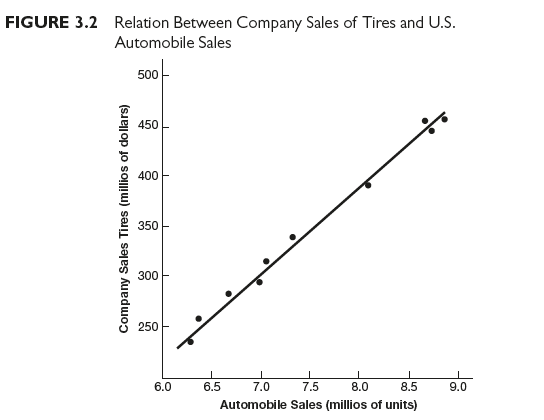
Computers make it easy to use regression analysis for sales forecasting. One tire manufacturer, for instance, used simple regression analysis to determine the association between economic variables and its own sales. This company discovered that a positive correlation existed between gross national product and its own sales, but the correlation coefficient was too low to use in forecasting company sales. The same was true of personal disposable income and retail sales; their correlation coefficients with company sales were too low to use in forecasting company sales. The tire manufacturer measured the relationship between its own dollar sales and unit sales of automobiles and found a much higher degree of correlation (see Figure 3.2). The dots on this scatter diagram cluster closely around the straight line that is the result of the mathematical computation between the two series of data. If the correlation had been perfect, all the dots would have fallen on the line.
Where sales are influenced by two or more independent variables acting together, multiple regression analysis techniques are applied. To illustrate, consider this situation. An appliance manufacturer is considering adding an automatic dishwasher to its line and decides to develop a forecasting equation for industry sales of dishwashers. From published sources, such as the Statistical Abstract of the United States, data are collected on manufacturers’ sales of dish washers for a period of twenty years (the dependent variable). Also collected are data on four possible independent variables:
- The Consumer Price Index for durables
- Disposable personal income deflated by the Consumer Price Index
- The change in the total number of households
- New nonfarm housing starts
Then, the analysts use stepwise multiple linear regression to estimate the relationship among the variables. Figure 3.3 shows the computer printout used in developing the forecasting equation. Here is a step-by-step explanation of the program output:
Step 1. Means and standard deviation for all variables:
X(l) is Consumer Price Index for durables (CPI).
X(2) is disposable personal income deflated by the Consumer Price Index (DPI/CPI).
X(3) is the change in the total number of households (DNH). X(4) is new nonfarm housing starts (NFHS).
X(5) is sales (the dependent variable).
Step 2. Simple pairwise correlation coefficients (note that sales volume is highly correlated with DPI/CPI and CPI).
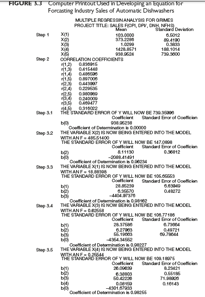
Step 3. Program enters independent variables in order of highest explained variation of the dependent variable:
- Program states distribution of dependent variable (sales) before the first independent variable is added.
- Variable X(2): DPI/CPI enters the model first. The standard error of Y is reduced to 147.209. The coefficient of determination is 0.96234; that is, X(2) explains approximately 96 percent of the variation in Y.
- Variable X(l): CPI enters the model next. (This means that X(l) explains the greatest portion of the variation in Y left over after the entry of X(2) in the model.) The standard error of Y is now reduced to 105.65553. The coefficient of multiple determination is increased to 0.98162.
- After the addition of variables X(2) and X(l), less than 2 percent of the variation in Y is left to be explained.
- The results of the additions of X(3) DNH and of X(4) NFHS indicate that these variables are not statistically significant; this is shown by the low F values as well as by the t values:
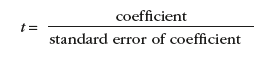
Therefore, the effect of adding these two variables to the model is not to reduce the standard error of Y but, in fact, in this case it is increased slightly.
These results indicate, then, that
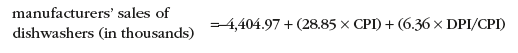
So if the manufacturer has estimates for the coming year that CPI will be 125 and DPI/CPI 550, its forecast of industry sales of dishwashers (in thousands) is
sales = -4.404.97 + (28.85)(125) + (6.36)(550)
= 2,699.28 (or approximately 2,700,000 dishwashers)
Evaluation of regression analysis for sales forecasting. If high coefficients of correlation exist between company sales and independent variables, the forecasting problem is simplified, especially if the variables “lead” company sales. The probable course of sales may then be charted, and the forecaster can concentrate on factors that might cause deviations. But it is necessary to examine other circumstances that might upset past relationships. A forecast made through regression analysis assumes that past relations will continue. A “lead-lag” association in which deviations regularly occur in related independent variable(s) prior to a change in company sales is a near-ideal situation, but it rarely holds except over short periods. Lead-lag relationships are common, but associations between the lead variables and sales in which the intervening time intervals remain stable are uncommon. Periods not only contract or expand erratically; they vary greatly during different phases of the business cycle.
If close associations exist between company sales and a reliable barometer, estimates are improved by experts’ predictions of probable changes in the barometer. However, one danger in using regression analysis is that forecasters may put too much faith in the statistical output. They may abandon independent appraisals of future events because of a statistically developed forecast. It is wrong to place blind faith in any forecasting method. It is wise to check results with those of other forecasts.
5. Econometric Model Building and Simulation
Econometric model building and simulation is attractive as a sales forecasting method for companies marketing durable goods. This approach uses an equation or system of equations to represent a set of relationships among sales and different demand-determining independent variables. Then, by “plugging in” values (or estimates) for each independent variable (that is, by “simulating” the total situation), sales are forecast. An econometric model (unlike a regression model) is based upon an underlying theory about relationships among a set of variables, and parameters are estimated by statistical analysis of past data. An econometric sales forecasting model is an abstraction of a real-world situation, expressed in equation form and used to predict sales. For example, the sales equation for a durable good can be written where
S = R +N
Where
S = total sales
R = replacement demand (purchases made to replace product units going out of use, as measured by the scrappage of old units)
N = new-owner demand (purchases made not to replace existing product units, but to add to the total stock of the product in users’ possession)
Total sales of a durable good, in other words, consist of purchases made to replace units that have been scrapped and purchases by new owners. Thus, a family that has a five-year-old machine trades it in to a dealer as part payment for a new machine and becomes part of the replacement demand (although only effectively so when the five-year- old machine, perhaps passing through several families’ hands in the process, finally comes to be owned by a family that goes ahead and consigns its even-older machine to the scrap heap).
Replacement demand is measured by the scrappage of old units of products, that is, by the percentage of the total stock of the product in users’ hands that is taken out of service through consignment to the trash pile, by sale to a junk dealer, or merely by being stowed away and never used again. Replacement demand in any one year does not include demand originating from the family that had a five-year-old machine that it traded to a dealer for a new machine, with the dealer reselling the old machine to another family who buys it secondhand. Only when a particular machine goes completely out of service is it regarded as scrapped, and, at that time (through a chain of purchases and trade-ins), some family becomes a part of replacement demand. Econometricians estimate replacement demand by using life expectancy of survival tables, which are similar to the life (or mortality) tables used by life insurance actuaries. An example is shown in Figure 3.4.
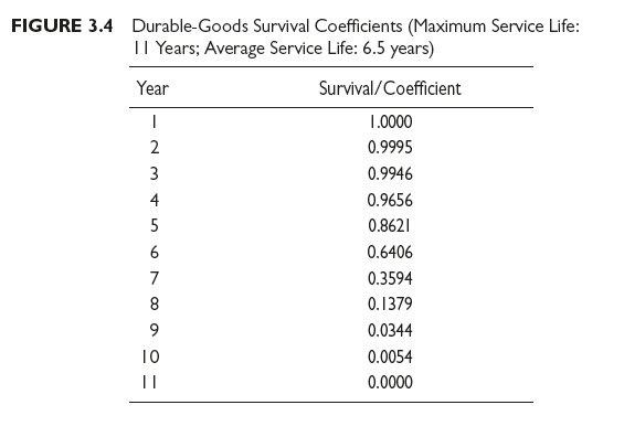
If some durable product has a maximum service life of eleven years and 10,000 units of the product enter service in some year, the table indicates that five years later, 8,621 will probably still be in service, and ten years later, 54. For this batch of 10,000 product units, scrappage is 1,035 in the fifth year (that is, 1,379 – 344, the difference between the accumulated total scrappage at the close of the fifth and fourth years, respectively). In the fifth year, then, 1,035 replacement sales trace back to the batch of 10,000 product units that entered service five years before.
New-owner demand is the net addition to users’ stocks of the product that occurs during a given period. For instance, if 2,000,000 units of some appliance were in service at the start of a period and 2,500,000 at the end, new-owner demand was 500,000 during the period. Forecasting the number of sales to new owners involves treating the stock of the product in the hands of users as a “population” exhibiting “birth” and “death” characteristics, that is, thinking of it as being analogous to a human population.
Constructing this sort of econometric model requires going through three steps. First, study independent variables affecting each demand category (replacement and new owner) and choose for correlation analysis those that bear some logical relationship to sales (the dependent variable). Second, detect that combination of independent variables that correlates best with sales. Third, choose a suitable mathematical expression to show the quantitative relationships among the independent variable[2] and sales, the dependent variables. This expression becomes the econometric model.
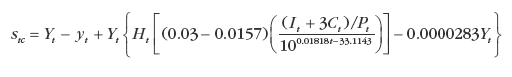
The procedure for building econometric models is simple, but finished models can take on formidable appearances. Consider, for example, this econometric model for forecasting sales of washing machines.[3]
where
Stc = calculated value for forecasted sales of washing machines during some time period Yt = level of consumers’ stock of washing machines in any period (as of January 1)
yt = level of consumers’ stock that would occur in the following period (as of January 1) if no washing machines were sold and scrappage rates remained the same
Ht = number of wired (i.e., electrified) dwelling units, in millions
It = disposable personal income
Ct = net credit extended (excluding credit extended for automobiles)
Pt = price index for house furnishings
![]()
Thus, new-owner demand in this model is represented by Yt – y , determined by applying appropriate survival coefficients to previous years’ sales of washing machines and estimating consumers’ total stocks of washing machines in each year. Replacement demand is represented by the other symbols in the equation and takes into account the number of wired dwelling units (washing machines are not sold to people who live in homes with no electricity), real purchasing power (disposable personal income plus credit availability divided by a price index), and real purchasing power adjusted for the historical trend. Regression analysis was used to derive the numerical values in this model.
Econometric model building seems a nearly ideal way to forecast sales. Not only does it consider the interaction of independent variables that bear logical and measurable relationships to sales, it uses regression analysis techniques to quantify these relationships. Econometric models, however, are best used to forecast industry sales, not the sales of individual companies. This is because the independent variables affecting an individual company’s sales are more numerous and more difficult to measure than are those determining the sates of an entire industry. Many companies use an econometric model to forecast industry sales, and then apply an estimate of the company’s share-of-the-market percentage to the industry forecast to arrive at a first approximation for the company’s forecasted sales.
Source: Richard R. Still, Edward W. Cundliff, Normal A. P Govoni, Sandeep Puri (2017), Sales and Distribution Management: Decisions, Strategies, and Cases, Pearson; Sixth edition.
The core of your writing whilst sounding agreeable initially, did not settle very well with me personally after some time. Somewhere within the sentences you managed to make me a believer unfortunately just for a short while. I however have got a problem with your jumps in assumptions and you would do nicely to help fill in those breaks. In the event that you can accomplish that, I would undoubtedly be amazed.