Operating Characteristic Curve

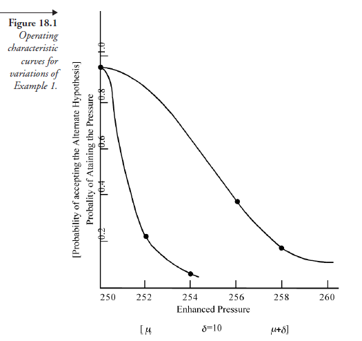
A given set of experimental situations can be represented in a graphical form, referred to as the operating characteristic curve for that set. To show how it is derived, we will revisit the design for experimental Situation Set 1.

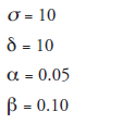
H0: μ1 = μ0 (average pressure, 250 psi)
(δ = 10; enhanced pressure, 260 psi)

In road testing the design, suppose 5 falls short of ten. It is quite possible that the experimenter will be satisfied with an increment of 8 psi instead, but he likes to know what the proba­bility of getting 258 psi is in the road test. And, what are the probabilities of getting 257, 256, 255, and so forth, just in case he can settle down to one of those? A graphical relation, known as the operating characteristic curve, which can help the experi­menter forecast answers to such questions, even before the road test, is our aim.

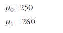
Now, we will look at the two formulas central in the design:

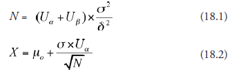
Between these two relations, the factors involved are μ0, σ, δ, Uα, Uβ,

X1, the mean of the enhanced pressure values, yet to be obtained from road testing the design, symbolized as μ1, and,

α and β, the risk factors, which, in turn, lead us respectively to Uα and Uβ (Table 18.2).

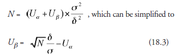
With these factors, the experimental Situation Set 1, in terms of numbers, reduces to

The enhanced pressures, 257, 256, and so forth, are simply the values of ^, its value becoming 260 with 6 = 10.

The operating characteristic curve, as mentioned earlier, is a graphical relation of probabilities for μ1 varying between 250 psi at one end and 260 psi at the other. The pressure 250 psi is given as an established fact for the design. It means the possibility of getting 250 psi is 100 percent. But because we have to contend with probabilities, not certainties, the possibility is less than 100 percent. What is the probability? The meaning of having chosen α = 0.05 is as follows: Although the pressure of 250 psi is an established fact, rejecting the null hypothesis amounts to asserting that there is bound to be an improvement in the pressure. This will be a statement in certainty, not probability. Conforming to probability, all that we can say is that there is a very high probability that this could happen. And that probability is (1 – α) = (1 – 0.05) = 0.95. If we plot pressure readings on the X-axis and probability on the Y-axis, there is a point withcoordinates X = 250, Y = 0.95. And, though we are not sure that there is an enhancement of 10 points in pressure (δ = 10, μ1 = 260), there is some possibility that this may happen; the probability of that is 0.10. Now we have the second point on the graph with coordinates X = 260 and Y = 0.10. We have probability numbers corresponding to the μ1 (enhanced pressures) = 250 and 260 psi. What is the probability number for an intermediate pressure, for example 256 (δ = 6) psi? To answer this, we will go to (18.1) above:

The operating characteristic curve, as mentioned earlier, is a graphical relation of probabilities for ^ varying between 250 psi at one end and 260 psi at the other. The pressure 250 psi is given as an established fact for the design. It means the possibil­ity of getting 250 psi is 100 percent. But because we have to contend with probabilities, not certainties, the possibility is less than 100 percent. What is the probability? The meaning of hav­ing chosen a = 0.05 is as follows: Although the pressure of 250 psi is an established fact, rejecting the null hypothesis amounts to asserting that there is bound to be an improvement in the pressure. This will be a statement in certainty, not probability. Conforming to probability, all that we can say is that there is a very high probability that this could happen. And that probabil­ity is (1 – a) = (1 – 0.05) = 0.95. If we plot pressure readings on the X-axis and probability on the Taxis, there is a point with coordinates X = 250, Y = 0.95. And, though we are not sure that there is an enhancement of 10 points in pressure (6 = 10, ^1 = 260), there is some possibility that this may happen; the proba­bility of that is 0.10. Now we have the second point on the graph with coordinates X = 260 and Y = 0.10. We have probabil­ity numbers corresponding to the ^1 (enhanced pressures) = 250 and 260 psi. What is the probability number for an inter­mediate pressure, for example 256 (6 = 6) psi? To answer this, we will go to (18.1) above:

In this formula, all the factors except 6 remaining unchanged, we can calculate the value of Uβ for δ = 6.

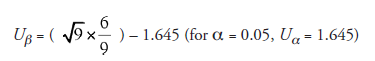
= 0.355 (assumption: all the road tests will be done with nine samples)

Now, going to Table 18.2, we can find (extrapolating), corre­sponding to Up = 0.355, the value of /3 to be 0.362.

This is the third point with coordinates X = 256 and Y = 0.362 on the probability curve. Calculations along similar lines for δ = 8 give us another point: X = 258, Y = 0.154. A bell-shaped (because it is normal distribution), smooth curve, drawn through these four points, gives the operating characteristic for this set of experimental conditions. For any given value of enhanced pressure in the range 250 to 260 (δ 0 – 10), for example, 254, the experimenter is able to find from this curve the probability of attaining it.

We note that for drawing this curve, we used (18.1) and (18.3), but made the assumption that N, the sample size, remained constant for all the road tests yet to be done. Instead, (18.1) can be used to find the sample size with varying increments in the dependent variable. For instance, with other data unchanged, the sample size, N, for δ = 4 is given as

N = (1.645 + 1.282)² x 10²/4² = 54

In the extreme case of δ = 1, a similar calculation gives us N = 857, an ungainly number for the sample size, particularly if each numerical value in the sample requires a replication. We notice that the difference we are considering in the response—the inde­pendent variable in this case, the pressure—is only 1 in 251. The implication is that situations in which minute changes in the response need to be detected require very large samples. The smaller the difference to be detected, the larger the sample required.

Suppose we take the sample size to be fifty-four, but keep the other variable factors the same in (18.3). Then, corresponding to δ = 4 and 2 (pressures 254 and 252), the values of β work out to be 0.0512 and 0.217, respectively. We can plot the points (x = 4, y = 0.0512) and (x = 2, y = 0.217). A bell-shaped, smooth curve passing through these points is good for sample size fifty-four only. Both these curves, one for N = 9 and another for N = 54, were obtained for conditions with a = 0.05. Now, if 5 is changed, the location and paths of the curves change too.

The curves, which show the probabilities of attaining, in steps, a given target for improvement, expressed in concrete terms of a problem, are often referred to as power curves. The same data may be expressed in general terms, namely: “Probability of accepting alternate hypothesis” on the Y-axis and “Increments of δ between μ0 and μ1” on the X-axis. Then, the curves are properly called the operating characteristic curves. Data from such curves can be applied to other problems with a comparable range of variables in experimental situations. Figure 18.1 shows these curves, alternatively to be called by either of the titles, depending on the way the X and the Y coordinates are expressed.

Finally, we take a closer look at (18.3), which is the basis for plotting the operating characteristics curve. It is a relation of probability Uβ to four variables:

1. The sample size, N
2. The intended increment
3. Uα, hence α
4. The standard deviation, α, which is likely to be known

The first three of these variables are interdependent. For example, by increasing N and decreasing δ, the value of Uβ can be kept
the same. Conversely, the value of Uβ can be changed by altering any one or more of N, δ, and Uα (hence α). Though these variables are situation specific, they are open to the discretion of the experimenter. A large number of graphical relations, connecting these variables to the probability of attaining the targeted improvements by experiments, are can be found in BiometrikaTables for Statisticians Vol 2, by E. S. Pearson and H. O. Hartle y, Cambridge University Press, Cambridge 1972. The reader is advised to refer to a standard text on “Design of Experiments,”

The first three of these variables are interdependent. For exam­ple, by increasing N and decreasing 5, the value of Up can be kept the same. Conversely, the value of Up can be changed by altering any one or more of N, 5, and U_a (hence a). Though these vari­ables are situation specific, they are open to the discretion of the experimenter. A large number of graphical relations, connecting these variables to the probability of attaining the targeted improvements by experiments, are can be found in Biometrika Tables for Statisticians Vol 2, by E. S. Pearson and H. O. Hartley, Cambridge University Press, Cambridge 1972. The reader is advised to refer to a standard text on “Design of Experiments,” many of which (e.g., D. C. Montgomery, Design and Analysis of Experiments, 5th ed. New York: John Wiley and Sons, 2001) con­tain selected adaptations of such data; these can be applied, with some interpolation, to specific experimental situations.

Source: Srinagesh K (2005), The Principles of Experimental Research, Butterworth-Heinemann; 1st edition.