Survival-Time Data in Stata

Survival-time data contain, at a minimum, one variable measuring how much time elapsed before a certain event occurred for each observation. The literature often terms this event of interest a “failure,” regardless of its real-world meaning. When failure has not occurred to an observation by the time data collection ends, that observation is said to be “censored.” The stset command sets up a dataset for survival-time analysis by identifying which variable measures time and (if necessary) which variable is a {0, 1} indicator for whether the observation failed or was censored. The dataset can also contain any number of other measurement or categorical variables. Individuals (for example, medical patients) can be represented by more than one observation.

To illustrate the use of stset, we will begin with an example from Selvin (1995:453) concerning 51 individuals diagnosed with HIV. The data initially reside in a raw-data file (aids.raw) that looks like this:

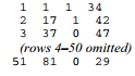
The first column values are case numbers (1, 2, 3, . . . , 51). The second column tells how many months elapsed after the diagnosis, before that person either developed symptoms of AIDS or the study ended (1, 17, 37, . . .). The third column holds a 1 if the individual developed AIDS symptoms (failure), or a 0 if no symptoms had appeared by the end of the study (censoring). The last column reports the individual’s age at the time of diagnosis.

We can read the raw data into memory using infile, then label the variables and data:

. infile case time aids age using C:\data\aids.raw, clear . label variable case “Case ID number”

. label variable time “Months since HIV diagnosis”

. label variable aids “Developed AIDS symptoms”

. label variable age “Age in years”

. label data “AIDS (Selvin 1995:453)”

. compress

The next step is to identify which variable measures time and which indicates failure/censoring. Although not necessary with these single-record data, we can also note which variable holds individual case identification numbers. In an stset command, the first-named variable measures time. Subsequently, we identify with failure) ) the dummy representing whether an observation failed (1) or was censored (0). After using stset, we save the dataset in Stata format to preserve this information.

stdescribe yields a brief description of how our survival-time data are structured. In this simple example we have only one record per subject, so some of this information is unneeded.

. stdescribe

The stsum command obtains summary statistics. We have 25 failures out of 3,164 person- months, giving an incidence rate of25/3164 = .0079014. The percentiles of survival time derive from a Kaplan-Meier survivor function (next section). This function estimates about a 25% chance of developing AIDS within 41 months after diagnosis, and 50% within 81 months. Over the observed range of the data (up to 97 months) the probability of AIDS does not reach 75%, so there is no 75th percentile given.

If the data happen to include a grouping or categorical variable such as sex, we could obtain summary statistics on survival time separately for each group by a command of the following form:

. stsum, by(sex)

Later sections describe more formal methods for comparing survival times from two or more groups.

Source: Hamilton Lawrence C. (2012), Statistics with STATA: Version 12, Cengage Learning; 8th edition.