Multiple Random Slopes by using Stata

To specify random coefficients on logdens, minority and colled we can simply add these variable names to the random-effects part of an xtmixed command. For later comparison tests, we save the estimation results with name full. Some of the iteration details have been omitted in the following output.

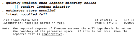
. xtmixed bush logdens minority colled

|| cendiv: logdens minority colled

Taking the full model as our baseline, likelihood-ratio tests establish that the random coefficients on logdens, minority and colled each have statistically significant variation, so these should be kept in the model. For example, to evaluate the random coefficients on colled we quietly estimate a new model without them (nocolled), then compare that model withfull. The nocolled model fits significantly worse (p ~ .0000) than the full model seen earlier.

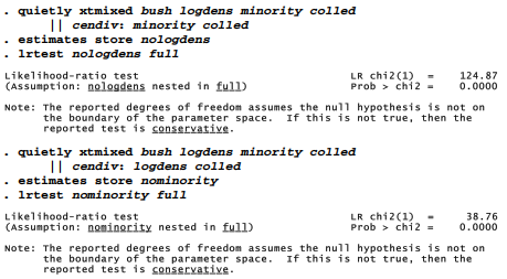
Similar steps with two further models (nologdens and nominority) and likelihood-ratio tests show that the full model also fits significantly better than models without either a random coefficient on logdens or one on minority.

We could investigate the details of all these random effects, or the combined effects they produce, through calculations along the lines of those shown earlier for Figure 13.5.

Mixed-modeling research often focuses on the fixed effects, with random effects included to represent heterogeneity in the data, but not of substantive interest. For example, our analysis thus far has demonstrated that population density, percent minority and percent college educated predict county voting patterns nationally, even after adjusting for regional differences in mean votes and for regional effects of density and college grads. On the other hand, random effects might themselves be quantities of interest. To look more closely at how the relationship between voting and percent college graduates (or percent minority, or log density) varies across census divisions, we can predict the random effects and from these calculate total effects. These steps are illustrated for the total effect of colled in our full model below, and graphed in Figure 13.6.

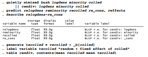
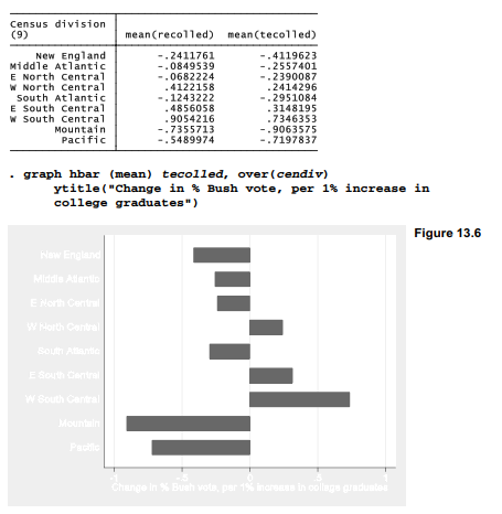
Figure 13.6 visualizes the reason our model was significantly improved (p ~ .0000) by including a random slope for colled. The total effects of colled on Bush votes range from substantially negative (percent Bush votes lower among counties with more college graduates) in the Mountain (-.91) and Pacific (-.72) census divisions, through negligible in the South Atlantic or W North Central, to substantially positive (+.73) in the W South Central where Bush votes were substantially higher in counties with more graduates — controlling for population density, percent minority and other regional effects. If we estimate only a fixed effect for colled, our model effectively would average these negative, near zero, and positive random effects of colled into one weakly negative fixed coefficient, specifically the -.18 coefficient in the two fixed- effects regressions that started off this chapter.

The examples seen so far were handled successfully by xtmixed, but that is not always the case. Mixed-model estimation can fail to converge for a variety of different reasons, resulting in repeatedly “nonconcave” or “backed-up” iterations, or error messages about Hessian or standard error calculations. The Longitudinal/Panel Data Reference Manual discusses how to diagnose and work around convergence problems. A frequent cause seems to be models with near-zero variance components, such as random coefficients that really do not vary much, or have low covariances. In such cases the offending components can reasonably be dropped.

Source: Hamilton Lawrence C. (2012), Statistics with STATA: Version 12, Cengage Learning; 8th edition.