1. Working with graphs
Stata has a rich system for graphical representation of data. The main command for creating graphs is unsurprisingly named graph. Behind this plain name is a wealth of tools. In this chapter, we will make one simple graph to point out the basics of the Graph window. See the [G] Stata Graphics Reference Manual for more information about all aspects of working with graphs.
2. A simple graph example
In the sample session of [GSW] 1 Introducing Stata—sample session, we made a scatterplot, added a fitted regression line, and made a grid of scatterplots to allow comparisons across groups. Here, using the automobile dataset, we make a simple box plot that shows the displacements of the cars’ engines and how they compare across repair records within the place of manufacture of the cars. Start by loading the dataset by typing sysuse auto in the Command window and pressing Enter.
We select Graphics > Box plot, choose or type displacement in the Variables field on the Main tab, click on the Categories tab, check the Group 1 checkbox and enter rep78 for the first grouping variable, and check the Group 2 checkbox and enter foreign for the second grouping variable. Finally, we click on the Submit button so that we could easily make changes to the graph if need be. After we look at the graph, we realize that we forgot the title. We close the Graph window, click on the Titles tab of the graph box dialog, type the title Displacement across repairs within origin, and click on the Submit button again.
The Graph window comes up, showing us our nicely titled graph:
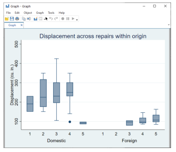
Graph window
When the Graph window comes up, it shows our graph in a window with a toolbar. The first four buttons are familiar to us from other Stata windows: Open, Save, Print, and Copy. The next two buttons are new:
![]() Rename graph: This button allows the graph to be renamed. Why would you do this? If you would like to have multiple graphs open at once, the graphs need to be named. So you can click on the Rename graph button to give a graph a name. This graph will then remain open when you create your next graph.
Rename graph: This button allows the graph to be renamed. Why would you do this? If you would like to have multiple graphs open at once, the graphs need to be named. So you can click on the Rename graph button to give a graph a name. This graph will then remain open when you create your next graph.
![]() Graph Editor: Stata has a Graph Editor that allows you to manipulate and edit your graph. This feature will be introduced in the next chapter.
Graph Editor: Stata has a Graph Editor that allows you to manipulate and edit your graph. This feature will be introduced in the next chapter.
The inactive buttons to the right of the Graph Editor button are used by the Graph Editor, so their meanings will become clear in the next chapter.
We decide that we like this graph and would like to save it. We can save it either by clicking on the Save button and choosing a name and a location or by right-clicking on the Graph window itself and selecting Save as
3. Saving and printing graphs
You can save a graph once it is displayed by right-clicking on its window and selecting Save as… You can print a graph by right-clicking on its window and selecting Print You can also use the File menu to save or print a graph. We recommend that you always right-click on a graph to save or print it to ensure that the correct graph is selected.
4. Right-clicking on the Graph window
Right-clicking on the Graph window displays a menu from which you can select the following:
- Save as… to save the graph to disk.
- Copy to copy the graph to the Clipboard.
- Start Graph Editor to start the Graph Editor.
- .. to edit the preferences for graphs.
- .. to print the graph.
5. The Graph button
The Graph button, ![]() , is located on the main window’s toolbar. The button has two parts, an icon and an arrow. Clicking on the icon brings the topmost Graph window to the front of all other windows. Clicking on the arrow displays a menu of open graphs. Selecting a graph from the menu brings that graph to the front of all other windows. If you close the Graph window, you can reopen it only by reissuing a Stata command that draws a new graph.
, is located on the main window’s toolbar. The button has two parts, an icon and an arrow. Clicking on the icon brings the topmost Graph window to the front of all other windows. Clicking on the arrow displays a menu of open graphs. Selecting a graph from the menu brings that graph to the front of all other windows. If you close the Graph window, you can reopen it only by reissuing a Stata command that draws a new graph.
Source: STATA (2021), Getting Started with Stata for Windows, Stata Press Publication.
1 Oct 2022
3 Oct 2022
3 Oct 2022
26 Sep 2022
28 Sep 2022
29 Sep 2022