Using the Data Editor in Stata

1. The Data Editor

The Data Editor gives a spreadsheet-like view of data that are currently in memory. You can use it to enter new data, edit existing data, search through the dataset, and edit attributes of the data in the dataset, such as variable names, labels, and display formats, as well as value labels.

In addition to the view of the data, there are two windows for manipulating variables and their properties: the Variables window and the Properties window. These are similar to the same-named windows in the main Stata window.

Any action you take in the Data Editor results in a command being issued to Stata as though you had typed it into the Command window. This means that you can keep good records and learn commands by using the Data Editor.

The Data Editor can be kept open while you work in Stata, giving you a live view of your dataset as you work. To protect your data from inadvertent changes, the Data Editor has two modes: edit mode for active editing and browse mode for viewing. In browse mode, editing within the Data Editor window is disabled. We highly recommend that you use the Data Editor in browse mode and switch to edit mode only when you want to make changes.

You can print your data from the Data Editor by selecting Print from the File menu.

We will be entering and editing data in this chapter, as well as manipulating the variables by using the Variables and Properties windows, so start the Data Editor in edit mode by clicking on the Data

Editor (Edit) button, PI.

2. Buttons on the Data Editor

The toolbar for the Data Editor has some standard buttons and some buttons we have not yet seen:

Edit mode: Changes the Data Editor to edit mode.

Browse mode: Changes the Data Editor to browse mode for safely looking at data.

Open: Opens a Stata dataset. Stata will warn you if your current dataset has unsaved changes.

Save: Saves the dataset visible in the Data Editor.

Print: Prints the dataset visible in the Data Editor.

Copy: Copies the current selection to the Clipboard.

Paste: Pastes the contents of the Clipboard. You may paste only if one cell is selected—this Cs cell will become the upper-left corner of the pasted contents. Warning: This action will paste over existing data.

Find: Opens the Find bar for searching in the Data Editor.

 Filter observations: Filters the observations visible in the Data Editor. This button is useful for looking at a subset of the current dataset.

You can move about in the Data Editor by using the typical methods:

• To move to the right, use the Tab key or the right arrow key.
• To move to the left, use Shift+Tab or the left arrow key.
• To move down, use Enter or the down arrow key.
• To move up, use Shift+Enter or the up arrow key.

You can also click within a cell to select it.

Right-clicking within the Data Editor brings up a contextual menu that allows you to manipulate the data and what you are viewing. Right-clicking on the Data Editor window displays a menu from which you can do many common tasks:

• Copy to copy data to the Clipboard.
• Paste to paste data from the Clipboard.
• Paste special… to paste data from the Clipboard with finer control of delimiters, giving a preview of what will be pasted.
• Select all to select all the data displayed in the Data Editor. This could be different from the data in the dataset if the data are filtered or some variables are hidden.
• Data to open a submenu containing
  • Insert variable… to bring up a dialog for creating a new variable at the current cursor position.
  • Add variable… to bring up a dialog for creating a new variable at the beginning or end of a dataset.
  • Replace contents of variable… to bring up a dialog for replacing the values of the selected variable.
  • Insert observations… to bring up a dialog for inserting new empty observations at the current cursor position.
  • Add observations… to bring up a dialog for adding new empty observations to the end of the dataset.
  • Sort data… to sort the dataset by the selected variable.
  • Value labels to access a submenu for managing and displaying value labels.
  • Keep only selected data to keep only the selected data in the dataset. All remaining data will be dropped (removed) from the dataset. As always, this affects only the data in memory. It will not affect any data on disk.
  • Drop selected data to drop the selected data. This is only possible if the selection consists of either entire variables (columns) or observations (rows).
  • Convert variables from string to numeric… for converting string variables to numeric variables, which is useful when the string variables contain characters for formatting numbers instead of just numbers.
  • Convert variables from numeric to string… for converting numeric variables to strings. • Encode string variable to labeled numeric… for encoding a string-valued categorical variable to a numeric variable while still displaying the categories in tables and graphs. • Decode labeled numeric variable to string… for turning an encoded variable back into a string variable.
• Reset selected column widths to reset the selected columns to the default width.
• Hide selected variables to hide the selected variables.
• Show only selected variables to hide all but the selected variables.
• Show entire dataset to turn off all filters and unhide all variables.
• Preferences.. to set the preferences for the Data Editor.
• Font .. to change the font of the Data Editor.

3. Data entry

Entering data into the Data Editor is similar to entering data into a spreadsheet. One major difference is that the Data Editor has the concept of observations, which makes the data entry smart. We will illustrate this with an example. It will be useful for you to follow the example at your computer. To work along, you will need to start with an empty dataset, so save your dataset if necessary, and then type clear in the Command window.

Note: As a check to see if your data have changed, type describe, short (or d,s for short). Stata will tell you if your data have changed.

Suppose that we have the following data, and we want to enter them into Stata:

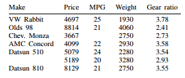
We do not know MPG for the third car or the make of the sixth.

Start by opening the Data Editor in edit mode. You can do this either by clicking on the Data

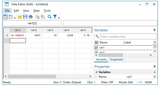
Editor (Edit) button, PI, or by typing edit in the Command window. You should be greeted by a Data Editor with no data displayed. (If you see data, type clear in the Command window.) Stata shows the active cell by highlighting it and displaying varname[obsnum] next to the input box in the Cursor Location box. We will see below that we can navigate within a dataset by using this cell reference. The Data Editor starts, by default, in the first row of the first column. Because there are no data, there are no variable names, and so Stata shows var1[1] as the active cell.

We can enter these data either by working across the rows (observation by observation) or by working down the columns (variable by variable). To enter the data observation by observation, press Tab after entering each value until you have reached the end of the first row. In our case, we would type VW Rabbit, press Tab, type 4697, press Tab, and continue entering data to complete the first observation.

After you are finished with the first observation, select the second cell in the first column, either by clicking within it or by navigating to it. At this point, your screen should look like this:

We can now enter the data for the second observation in the same fashion as the first—with one nice difference: after we enter the last value in the row, pressing the Tab key will bring us to the first cell in the third row. This is possible because the number of variables is known after the first observation has been entered, so Stata knows when it has all the data for an observation.

We can enter the rest of the data by pressing the Tab key between entries, simply skipping over missing values by tabbing through them.

If we had wanted to enter the data variable by variable, we could have done that by pressing Enter between each make of car until all seven observations were entered, skipping past the missing entry by pressing Enter twice. Once the first variable was entered, we would select the first cell in the second column and enter the price data. We would continue this until we were finished.

4. Notes on data entry

There are several things to note about data entry and the feedback you get from the Data Editor as you enter data:

• Stata does not allow blank columns or rows in the middle of your dataset.

Whenever you enter new variables or observations, always begin in the first empty column or row. If you skip columns or rows, Stata will fill in the intervening columns or rows with missing values.

• Strings and value labels are color coded.

To help distinguish between the different types of variables in the Data Editor, string values, value labels (see [GSW] 9 Labeling data), and all other values are displayed in different colors. You can change the colors for strings and value labels by right-clicking on the Data Editor window and selecting Preferences…………

• A period (.) represents Stata’s system missing numeric value.

Stata has a system missing value, ‘.’, and extended missing values ‘.a’ through ‘.z’. By default, Stata uses its system missing value.

• The Tab key is smart.

As we saw above, after the first observation has been entered, Stata knows how many variables you have. So at the end of the second observation (and all subsequent observations), Tab will automatically take you back to the first column.

• The Cursor Location box both shows location and is used for navigation.

The Cursor Location box gives the location of the current cell. If you see, for example, var3[4], this means that the current cell is the fourth observation of the variable named var3. You can navigate to a particular cell by typing the variable name and the observation in the Cursor Location box. If you wanted the second observation of varl to be the active cell, typing varl 2 in the Cursor Location box and pressing Enter would take you there.

• Double quotes around text are unnecessary in string variables.

Once Stata knows that a variable is a string variable (it holds text), there is no need to put quotes around the values, even if the values look like a number. Thus, if you wanted to enter ZIP codes as text, you would enter the first ZIP code with quotes (“02173”), but the rest would not need any quotes.

• The arrow keys are context sensitive.

If you select a cell and type new data, using an arrow key will accept the change and move to a new active cell. If you double-click on a cell, you can edit within the cell contents. In this case, the right- and left-arrow keys move within the cell’s data.

• You can throw away changes to a cell.

If, while you are entering data in a cell, you decide you would like to cancel the changes, press the Esc key or click outside the cell.

5. Renaming and formatting variables

The data have now been entered into Stata, but the variable names leave something to be desired: they have the default names varl, var2, …, var5. We would like to rename the variables so that they match the column titles from our dataset. We would also like to give the variables descriptions and change their formatting.

We will step through changing the name, label, and format of the price variable. We will then add a note to the variable. Start by clicking on the var2 variable in the Variables window. The few properties associated with var2 are now visible and editable in the Properties window. We may now systematically change the properties of var2 to our choosing:

1. Double-click on var2 in the Name field to select the old variable name, and type price to overwrite the name.
2. Click under the new price name in the Label
3. Enter a worthwhile label, such as Price in dollars.
4. Click on %9.0g in the Format
5. Click on the ellipsis (…) button that appears. The Create format dialog opens.
6. You can see here that there are many possible formats, most of which are related to time. We want commas in our numbers, so check the Use commas in numeric output When you are done, click on the OK button.
7. Click in the Notes
8. Click on the ellipsis (…) button that appears. A dialog called Notes for price
9. Click on the Add button and type a clever note.
10. When you are done typing, click on the Submit button, and then click on the Close This note is now attached to the price variable.
11. Click on the disclosure control to see the note you just typed in the Properties window.

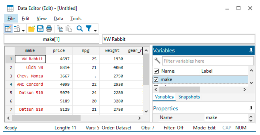
To edit the properties of another variable, click on the variable in the Variables window. We can name the first variable make; the third, mpg; the fourth, weight; and the fifth, gear_ratio. Just before you rename var5 to gear_ratio, your screen should look like this:

You need to know some rules for variable names:

• Stata is case sensitive.

Make, make, and MAKE are all different names to Stata. If you had named your variables Make, Price, MPG, etc., then you would have to type them correctly capitalized in the future. Using all lowercase letters is easier.

• A variable name must be 1-32 characters long.
• The characters can be letters (A-Z, a-z), digits (0-9), underscores (_), or Unicode characters that are not symbols.
• Spaces or other characters are not allowed.
• The first character of a variable name must be a letter, an underscore, or a Unicode character. Although you can use an underscore to begin a variable name, it is highly discouraged. Such names are used for temporary variable names in Stata. You would like your data to be permanent, so using a temporary name could lead to great frustration.

For more information about variable names and value labels, see [GSW] 9 Labeling data; for display formats, see [U] 12.5 Formats: Controlling how data are displayed.

6. Copying and pasting data

You can copy and paste data by using the Data Editor. This is often a simple way to bring data into Stata from any other applications such as spreadsheets or databases.

1. Select the data that you wish to copy by using one of these means:

• Click once on a variable name or column heading to select an entire column.
• Click once on an observation number or row heading to select the entire row.
• Click and drag the mouse to select a range of cells.

2. Copy the data to the Clipboard by right-clicking within the selected range, and select Copy.
3. Paste the data from the Clipboard by right-clicking on the top left cell of the area to which you wish to paste, and select Paste.

We will illustrate copying and pasting an observation by making a copy of the first observation and pasting it at the end of the dataset.

Start by clicking on the observation number of the first observation. Doing so highlights all the data in the row. Right-click on the same location (there is no need to move the mouse), and select Copy:

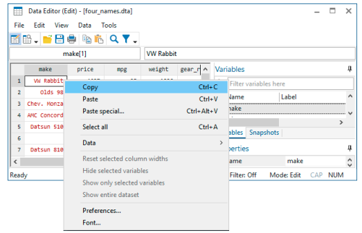
Click on the first cell in the eighth row, right-click while you are still in that cell, and choose Paste from the resulting menu. You can see that the observation was successfully duplicated.

7. Notes on copying and pasting

• The above example illustrated copying and pasting within the Data Editor. You can use roughly the same technique to copy and paste between other applications and Stata and between Stata and other applications. The easiest way to see if copying and pasting works properly with another application is to try it. The one requirement for things to work well is that the external application must copy tables in some delimited form, as do spreadsheet applications, many database applications, and some word processors. Using Edit > Paste special… gives some added flexibility to the formats you can paste into the Data Editor. If a simple paste does not give you what you expected, you should try Edit > Paste special  For more information on file-based methods for importing data into Stata, see [GSW] 8 Importing data.

• If you are copying and pasting data with value labels, you have a choice. You can copy variables with value labels as text, using the value labels as the actual values, or you can copy said variables as their underlying encoded numbers. Copying with the value labels is the default. If you would like the other choice, right-click in the Data Editor and select Data > Value labels > Hide all value labels, or select Tools > Value labels > Hide all value labels.

8. Changing data

As its name suggests, the Data Editor can be used to edit your dataset. As we have seen already, it can be used to edit the data themselves as well as the description and display options for the variables.

Here is an example for making some changes to the automobile dataset, which illustrates both methods for using the Data Editor and its documentation trail. We will also keep snapshots of the dataset as we are working so that we can revert to previous versions of the dataset in case we make a mistake.

We would like to investigate the dataset, work with value labels, delete the trunk variable, and make a new variable showing gas consumption per 100 miles. These tasks will illustrate the basics of working in the Data Editor.

Start by typing sysuse auto into the Command window. If you worked the previous example, you will get an error and are told that the dataset in memory has changed since it was last saved. This is good—Stata is keeping you from inadvertently throwing away the unsaved changes to your current dataset as it loads auto.dta. If you would like to save the dataset you have been working on, select File > Save and save the dataset in an appropriate location. Otherwise, type clear in the Command window, and press Enter to clear out the data, and then load that auto.dta.

Once auto.dta is loaded, start the Data Editor.

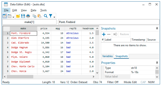
1. We remember that our grandfather had a Toronado, which looked sleek but seemed to require a lot of fill-ups. We would like to see if this car is in the dataset. To find it, we select Edit > Find…, type Toronado, and press Enter. We see that this make of car got 16 miles per gallon.
2. We would like to see which cars have the lowest and highest gas mileages. To do this, right-click on the column heading of the mpg Select Data > Sort data… from the contextual menu. A dialog will pop up asking how you want to sort, defaulting to sorting in ascending order. Click on OK. (Stata worries about sort order because sort order can affect reproducibility when using resampling techniques. This is a good thing.) You will see that the data have now been sorted by mpg in ascending order. The lowest-mileage cars are at the top of the screen; by scrolling to the bottom of the dataset, you can find the highest-mileage cars. You also could have sorted by selecting Tools > Sort data… once the mpg variable was selected.
3. We would like to investigate repair records and hence sort by the rep78 (Do this now.) We see that the Starfire and Firebird both had poor repair records, but we would like to see the cars with good repair records. We could scroll to the bottom of the dataset, but it will be faster to use the Cursor Location box: type rep78 74 and press Enter to make rep78[74] the active cell. We notice that the last five entries for rep78 appear as dots. The dots mean that these values are missing. A few items of note:

• • As we can see from the result of the sort, Stata views missing values as being larger than all numeric nonmissing values. In technical terms, this means that rep78 >= . is equivalent to missing(rep78).
  • What we do not see here is that Stata has multiple missing-value indicators: . is Stata’s default or system missing-value indicator, and .a, .b, …, .z are Stata’s extended missing values. Extended missing values are useful for indicating the reason why a value is unknown.
  • The different missing values sort among themselves: . < .a < .b < ••• < .z. See [U] 12.2.1 Missing values for full details.

4. We would like to make the repair records readable. Click on rep78 in the Variables window.
5. Click on the Value label field in the Properties window, and then click on the ellipsis (…) button that appears. This opens the Manage value labels We need to define a new value label for the repair records.
   • Click on the Create label You will see the Create label dialog.
   • Type a name for the label, say, repairs, in the Label name
   • Press the Tab key or click within the Value field.
   • Type 1 for the value, press the Tab key, and type atrocious for the label.
   • Press the Enter key to create the pairing.
   • Repeat steps d and e to make all the pairings: 2 with “bad”, 3 with “OK”, 4 with “good”, and 5 with “stupendous”.
   • Click on the OK button to finish creating the value label.
   • Click on the disclosure control, ±J to show the label—you should see this:

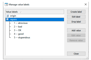
If you have something else, you can edit the label by clicking on the Edit label button.

1. • Click on the Close button to close the Manage value labels dialog.

Now that the label has been created, attach it to the rep78 variable by clicking on the down arrow in the Value label field and selecting the repairs label. You can now see the labels displayed in place of the values.

6. Suppose that we found the original source of the data in a time capsule, so we could replace some of the missing values for rep78. We could type the values into cells. We can also assign the values by right-clicking within a cell with a missing value and choosing a value from Data > Value labels > Assign value from value label “repairs”. This strategy can be useful when a value label has many possible values.
7. We would now like to delete the trunk variable. We can do this by right-clicking on the trunk variable name at the top of the column and selecting the Data > Drop selected data menu item. Because this can lead to data loss, the Data Editor asks whether we would like to drop the selected variable. Click on the Yes
8. To finish up, we would like to create a variable containing the gallons of gasoline per 100 miles driven for each of the cars.
   • Right-click within any cell, and choose the Data > Add variable… menu item to bring up the generate
   • Type gp100m in the Variable name
   • Being sure that the Specify a value or an expression radio button is selected, type 100/mpg in its field. We could have clicked on the .. button to open the Expression Builder dialog, but this formula was simple enough to type. (You might want to explore the Expression Builder right now to see what it can do.)
   • Be sure that the Add at the end of dataset item is chosen from the Position of new variable
   • Click on OK. You can scroll to the right to see the newly created variable.

Throughout this data-editing session, we have been using the Data Editor to manipulate the data. If you look in the Results window, you will see the commands and their output. You can also see all the commands generated by the Data Editor in the History window. If you wanted to save the editing commands to use again later, you could do the following steps:

1. Click in the History window on the last command that came from the Data Editor.
2. Scroll up until you find the sort mpg command you ran immediately after opening the Data Editor, and Shift-click on it.
3. Right-click on one of the highlighted commands.
4. Select Send selected to Do-file Editor.

This procedure will save all the commands you highlighted into the Do-file Editor. You could then save them as a do-file, which you could run again later. We will talk more about the Do-file Editor in [GSW] 13 Using the Do-file Editor—automating Stata. You can find help about do-files in [U] 16 Do-files.

If you want to save this dataset, save it under a new name by using File > Save as… in the main Stata window to prevent overwriting the original dataset.

9. Working with snapshots

The Data Editor allows you to save to disk snapshots of whatever dataset you are working on. These are temporary copies of the dataset—they will be deleted when you exit Stata, so they need to be treated as temporary. Still, there are many uses for snapshots, such as

• saving a temporary copy of the data in memory so that another dataset can be opened and viewed;
• saving stages of work, which can be recovered in case you do something disastrous; and
• saving pieces of datasets while doing analyses.

We will keep using auto.dta from above; if you are starting here, you can start fresh by typing sysuse auto in the Command window to open the dataset. (If you get a warning about data in memory being lost, either use clear or save your data. See [GSW] 5 Opening and saving Stata datasets for more information.) If we open the Data Editor and click on the Snapshots tab beneath the Variables window, we see the following window. If you are starting afresh, you will see numbers rather than labels for rep78.

To begin with, only one button is active in the Snapshots toolbar. Click on the active button—the

Add button, . It brings up a dialog asking for a label, or name, for the snapshot. Give it an inventive name, such as Start, and press Enter. You can see that a snapshot is now listed in the Snapshots window, and all the buttons in the toolbar are now active. The following buttons appear in the Snapshots window:

Add: Save a new snapshot with a timestamp and label.

Remove: Erase a snapshot. This action deletes the temporary snapshot file but does not affect the data in memory.

Change label: Edit the label of the selected (highlighted) snapshot.

Restore: Replace the data in memory with the data from the selected snapshot. You will get a dialog asking you to confirm your action.

You should now try manipulating the dataset by using the tools we have seen. Once you have done that, create another snapshot, calling it Changed. Open the Snapshots window and restore the Start snapshot by either double-clicking it or clicking first on it and then on the Restore button to see where you started. You can then go back to where you were working by restoring your Changed snapshot.

Snapshots continue to be available either until they are deleted or until you exit Stata. You can thus use snapshots of one dataset while working on another. You will find your own uses for snapshots—just take care to save the datasets you want for future use because the snapshots are temporary.

10. Dates and the Data Editor

The Data Editor has two special tools for working with dates in Stata. To see these in action, we will need to open another dataset. Either save your dataset or clear it out, and then type sysuse sp500 in the Command window. Look in the Data Editor to see what you have.

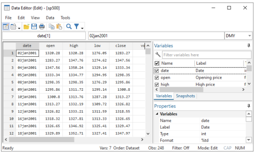
You can see a date variable that has January 2, 2001, as its first day, though it is being displayed in Stata’s default format for dates.

We will start with formatting:

1. Select the date variable in the Variables window to the right of the data table.
2. In the Properties window, select the Format row and click on the ellipsis button that appears.
3. The Create format dialog tells us three pieces of information about the date format:

• These are daily dates. As you can see, Stata understands other types of dates that are often used in financial data.
• Looking at the bottom of the dialog, you can see that Stata’s default date format is %td. This means that the variable contains time values that are to be interpreted as daily dates.
• This default format is displayed as, for example, 07apr2021.

4. There are many premade date formats in the Samples pane at the top right of the Create format Click on April 7, 2021. You can see how the format would be specified at the bottom of the dialog.
5. Click on OK to close the Create format You can see that the dates are now displayed differently.

This is a very simple way to change date formats. For complete information on dates and date formats, see [D] Datetime.

We will now change some of the dates to illustrate how this can be done simply, regardless of the format in which the dates are displayed. If you look in the upper-right corner of the Data Editor, you will see the Time/Date input mask field, which shows DMY. This field affects how dates are entered when editing data.

By default, the input mask is set to DMY. This means dates can be entered in many different fashions, as long as the order of the date components is day, month, year. Try the following:

1. Click in the first observation of date so that the Cursor Location shows date[1].
2. Type 18jan2021 and press the Enter Stata understands the DMY input mask and knows enough to enter the new date in the selected cell.
3. Enter 30042021 and press Stata still understands the input mask, even though there are no separators.
4. Click within the Time/Date input mask field, and choose MDY from the drop-down menu.
5. Click on any observation in the date column.
6. Type March 15, 2021 and press Enter. Stata will still understand.

Working in this fashion is the fastest way to edit dates by hand. If you look in the Results window, you will see why.

We are now finished with this dataset, so type clear and press Enter.

11. Data Editor advice

As you could see above, a small mistake in the Data Editor could cause large problems in your dataset. You really must take care in how you edit your data.

• People who care about data integrity know that editors are dangerous—it is easy to accidentally make changes. Never use the Data Editor in edit mode when you just want to look at your data. Use the Data Editor in browse mode (or use the browse command).

• If you must edit your data, protect yourself by limiting the dataset’s exposure. For example, if you need to change rep78 only if it is missing, find a way to look at just the missing values for rep78 and any other variables needed to make the change. This will make it impossible for you to change (damage) variables or observations other than those you view. We will explore this aspect shortly.
• Even with these caveats, Stata’s Data Editor is safer than most because it records commands in the Results window. Use this feature to log your output and make a permanent record of the changes. Then you can verify that the changes you made are the changes you wanted to make. See [GSW] 16 Saving and printing results by using logs for information on creating log files.

12. Filtering and hiding

We would now like to investigate restricting our view of the data we see in the editor. This feature is useful for the reasons mentioned above, and as we will see, it helps if we would like to browse through the data of a large dataset. In any case, we would like to focus on some data, not all the data, whether we focus on some of the variables, some of the observations, or even just some observations within some variables. We would also like to change the order of the variables. We will show you how this is done by using both the graphical interface and commands.

Open the automobile dataset by typing sysuse auto. If you get an error message, type clear and try again. Once you have done that, open the Data Editor.

Suppose that we would like to edit only those observations for which rep78 is missing. We will need to look at the make of the car so that we know which observations we are working with, but we do not need to see any other variables. We will work as though we had a very large dataset to work with.

1. Before we get started, try experimenting with the Variables window.
   • Drag variables up and down the list. Doing so changes the order of the variables’ columns in the Data Editor. It does not change their order in the dataset itself.
   • Uncheck some of the checkboxes in the first column to hide some of the variables.
   • Type a search criterion in the Filter variables here Just like in the Variables window in the main Stata window, the default is to ignore case and find any variables or variable labels containing any of the words in the filter. Clicking on the wrench on the left will allow you to change this behavior as well as to add or remove additional columns containing information about the variables. The filtering of variables in the list affects what is displayed in the Variables window; it does not affect what variables’ data are displayed. When you are done, delete your filter text.
2. Right-click on any variable in the Variables window, and select Select all from the contextual menu.
3. Click on any checkbox to deselect all the variables.
4. Click on the make variable to select it, and deselect all the other variables.
5. Click on the checkbox for make.
6. Click on the checkbox for rep78.

If you look in the Command window, you can see that no commands have been issued, because hiding the variables does not affect the dataset—it affects only what shows in the Data Editor.

We now have protected ourselves by using only those variables that we need. We should now reduce our view to only those observations for which rep78 is missing. This is simple.

1. Click on the Filter observations button, , in the Data Editor’s toolbar.
2. Enter missing(rep78) in the Filter by expression
3. Click on the Apply filter
4. If you are curious, click on the ellipsis button. It opens up an Expression Builder This lists the wide variety of functions available in Stata. See the Stata Functions Reference Manual.

Now we are focused on the part of the dataset in which we would like to work, and we cannot destroy or mistakenly alter other data by stray keystrokes in the Data Editor window.

It is worth learning how to hide variables and filter observations in the Data Editor from the Command window. This can be quite convenient if you are going to restrict your view, as we did above. To work from the Command window, we must use the edit command together with a varlist (variable list) along with if and in qualifiers in the Command window. By using a varlist, we restrict the variables we look at, whereas the if and in qualifiers restrict the observations we see. ([GSW] 10 Listing data and basic command syntax contains many examples of using a command with a variable list and if and in.) Suppose we want to correct the missing values for rep78. The minimum amount of data we need to expose are make and rep78. To see this minimal amount of information and hence to minimize our exposure to making mistakes, we enter the commands

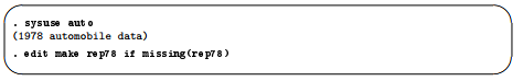
and we would see the following window:

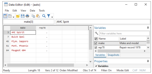
Once again, we are safe and sound.

Keep this lesson in mind if you edit your data. It is a lesson well learned.

13. Browse mode

The purpose of using the Data Editor in browse mode is to look at data without altering them by stray keystrokes. You can start the Data Editor in browse mode by clicking on the Data Editor

(Browse) button, , or by typing browse in the Command window. When you work in browse mode, all contextual menu items that would let you alter the data, the labels, or any of the display formats for the variables are disabled. You may view a variable’s properties with the Properties menu item, but you may not make any changes. You still can filter observations and hide variables to get a restricted view because these actions do not change the dataset.

Note: Because you can still use Stata menus not related to the Data Editor and because you can still type commands in the Commands window, it is possible to change the data even if the Data Editor is in browse mode. In fact, this means you can watch how your commands affect the dataset. You are merely restricted from using the Data Editor itself to change the data.

Source: STATA (2021), Getting Started with Stata for Windows, Stata Press Publication.