The Abandonment Option

Expansion value is important. When investments turn out well, the quicker and easier the business can be expanded, the better. But suppose bad news arrives, and cash flows are far below expectations. In that case, it is useful to have the option to bail out and recover the value of the project’s plant, equipment, or other assets. The option to abandon is equivalent to a put option. You exercise that abandonment option if the value recovered from the project’s assets is greater than the present value of continuing the project for at least one more period.

1. Bad News for the Perpetual Crusher

We introduced the perpetual crusher project in Chapter 19 to illustrate the use of the weighted- average cost of capital (WACC). The project cost $12.5 million and generated expected per­petual cash flows of $1.175 million per year. With WACC = .094, the project was worth PV = 1.175/.094 = $12.5 million. Subtracting the investment of $12.5 million gave NPV = 0.

Several years later, the crusher has not panned out. Cash flows are still expected to be perpetual but are now running at only $450,000 a year. The crusher is therefore worth only $450,000/.094 = $4.8 million. Is this bad news terminal?

Suppose the crusher project can be abandoned, with recovery of $5.2 million from the sale of machinery and real estate. Does abandonment make sense? The immediate gain from abandonment is of course $5.2 – 4.8 = $.4 million. But what if you can wait and reconsider abandonment later? In this case, you have an abandonment option that does not have to be exercised immediately.

We can value the abandonment option as a put. Assume for simplicity that the put lasts one year only (abandon now or at year 1) and that the one-year standard deviation of the crusher proj­ect is 30%. The risk-free interest rate is 4%. We value the one-year abandonment put using the Black-Scholes formula and put-call parity. The asset value is $4.8 million and the exercise price is $5.2 million. (See Section 21-3 if you need a refresher on using the Black-Scholes formula.)

Call value = .49 million or $490,000 (from the Black-Scholes formula)

      Put value = call value + PV (exercise pr ice) – asset value (put-call parity)

= .49 + (5.2/1.04) – 4.8 = .690, or $690,000

Therefore, you decide not to abandon now. The project, if alive, is worth 4.8 + .690 = $5.49 million when the abandonment put is included but only $5.2 million if it is abandoned immediately.

You are keeping the project alive not out of stubbornness or loyalty to the crusher, but because there is a chance that cash flows will recover. The abandonment put still protects on the downside if the crusher project deals up further disappointments.

Of course, we have made simplifying assumptions. For example, the recovery value of the crusher is likely to decline as you wait to abandon. So perhaps we are using too high an exer­cise price. On the other hand, we have considered only a one-year European put. In fact, you have an American put with a potentially long maturity. A long-lived American put is worth more than a one-year European put because you can abandon in year 2, 3, or later if you wish.

2. Abandonment Value and Project Life

A project’s economic life can be just as hard to predict as its cash flows. Yet NPVs for capital-investment projects usually assume fixed economic lives. For example, in Chapter 6 we assumed that the guano project would operate for exactly seven years. Real-option tech­niques allow us to relax such fixed-life assumptions. Here is the procedure:

1. Forecast cash flows well beyond the project’s expected economic life. For example, you might forecast guano production and sales out to year 15.
2. Value the project, including the value of your abandonment put, which allows, but does not require, abandonment before year 15. The actual timing of abandonment will depend on project performance. In the best upside scenarios, project life will be 15 years—it will make sense to continue in the guano business as long as possible.

In the worst downside scenarios, project life will be much shorter than 7 years.

In intermediate scenarios where actual cash flows match original expectations, abandonment will occur around year 7.

This procedure links project life to the performance of the project. It does not impose an arbi­trary ending date, except in the far distant future.

3. Temporary Abandonment

Companies are often faced with complex options that allow them to abandon a project temporarily—that is, to mothball it until conditions improve. Suppose you own an oil tanker operating in the short-term spot market. (In other words, you charter the tanker voyage by voyage, at whatever short-term charter rates prevail at the start of the voyage.) The tanker costs $50 million a year to operate, and at current tanker rates, it produces charter revenues of $52.5 million per year. The tanker is therefore profitable but scarcely cause for celebration. Now tanker rates dip by 10%, forcing revenues down to $47.5 million. Do you immediately lay off the crew and mothball the tanker until prices recover? The answer is clearly yes if the tanker operation can be turned on and off like a faucet. But that is unrealistic. There is a fixed cost to mothballing the tanker. You don’t want to incur this cost only to regret your decision next month if rates rebound to their earlier level. The higher the costs of mothballing and the more variable the level of charter rates, the greater the loss that you will be prepared to bear before you call it quits and lay up the boat.

Suppose that eventually you do decide to take the boat off the market. You lay up the tanker temporarily.^[2] Two years later, your faith is rewarded; charter rates rise, and the rev­enues from operating the tanker creep above the operating cost of $50 million. Do you reac­tivate immediately? Not if there are costs to doing so. It makes more sense to wait until the project is well in the black and you can be fairly confident that you will not regret the cost of bringing the tanker back into operation.

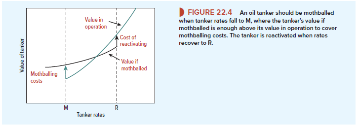
These choices are illustrated in Figure 22.4. The teal line shows how the value of an oper­ating tanker varies with the level of charter rates. The black line shows the value of the tanker when mothballed.^[3] The level of rates at which it pays to mothball is given by M and the level at which it pays to reactivate is given by R. The higher the costs of mothballing and reactivat­ing and the greater the variability in tanker rates, the farther apart these points will be. You can see that it will pay for you to mothball as soon as the value of a mothballed tanker reaches the value of an operating tanker plus the costs of mothballing. It will pay to reacti­vate as soon as the value of a tanker that is operating in the spot market reaches the value of a mothballed tanker plus the costs of reactivating. If the level of rates falls below M, the value of the tanker is given by the black line; if the level is greater than R, value is given by the teal line. If rates lie between M and R, the tanker’s value depends on whether it happens to be mothballed or operating.

Source:  Brealey Richard A., Myers Stewart C., Allen Franklin (2020), Principles of Corporate Finance, McGraw-Hill Education; 13th edition.