We now turn to an alternative way to take account of financing decisions. This is to calculate an adjusted present value or APV. The idea behind APV is to divide and conquer. Instead of capturing the effects of financing by adjusting the discount rate, APV makes a series of present value calculations. The first calculation establishes a base-case value for the project or firm: its value as a separate, all-equity-financed venture. The discount rate for the base- case value is just the opportunity cost of capital. Once the base-case value is set, then each financing side effect is traced out, and the present value of its cost or benefit to the firm is calculated. Finally, all the present values are added together to estimate the project’s total contribution to the value of the firm:
APV = base-case NPV + sum of PVs of financing side effects22
The most important financing side effect is the interest tax shield on the debt supported by the project (a plus). Other possible side effects are the issue costs of securities (a minus) or financing packages subsidized by a supplier or government (a plus).
APV gives the financial manager an explicit view of the factors that are adding or subtracting value. APV can prompt the manager to ask the right follow-up questions. For example, suppose that base-case NPV is positive but less than the costs of issuing shares to finance the project. That should prompt the manager to look around to see if the project can be rescued by an alternative financing plan.
1. APV for the Perpetual Crusher
APV is easiest to understand in simple numerical examples. Let’s apply it to Sangria’s perpetual crusher project. We start by showing that APV is equivalent to discounting at WACC if we make the same assumptions about debt policy.
We used Sangria’s WACC (9.4%) as the discount rate for the crusher’s projected cash flows. The WACC calculation assumed that debt will be maintained at a constant 40% of the future value of the project or firm. In this case, the risk of interest tax shields is the same as the risk of the project.[1] Therefore, we can discount the tax shields at the opportunity cost of capital (r). We calculated the opportunity cost of capital in the last section by unlevering Sangria’s WACC to obtain r = 9.9%.
The first step is to calculate base-case NPV. This is the project’s NPV with all-equity financing. To find it, we discount after-tax project cash flows of $1.175 million at the opportunity cost of capital of 9.9% and subtract the $12.5 million outlay. The cash flows are perpetual, so
![]()
Thus, the project would not be worthwhile with all-equity financing. But it actually supports debt of $5 million. At a 6% borrowing rate (rD = .06) and a 21% tax rate (Tc = .21), annual tax shields are .21 x .06 x 5 = .063, or $63,000.
What are those tax shields worth? If the firm is constantly rebalancing its debt, we discount at r = 9.9%:
![]()
APV is the sum of base-case value and PV(interest tax shields):
APV = −0.63 million + 0.63 million = 0
This is exactly the same as we obtained by one-step discounting with WACC. The perpetual crusher is a break-even project by either valuation method.[2]
But with APV, we don’t have to hold debt at a constant proportion of value. Suppose Sangria plans to keep project debt fixed at $5 million. In this case, we assume the risk of the tax shields is the same as the risk of the debt and we discount at the 6% rate on debt:
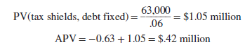
Now the project is more attractive. With fixed debt, the interest tax shields are safe and therefore worth more. (Whether the fixed debt is safer for Sangria is another matter. If the perpetual crusher project fails, the $5 million of fixed debt may end up as a burden on Sangria’s other assets.)
2. Other Financing Side Effects
Suppose Sangria has to finance the perpetual crusher by issuing debt and equity. It issues $7.5 million of equity with issue costs of 7% ($.53 million) and $5 million of debt with issue costs of 2% ($.10 million). Assume the debt is fixed once issued, so that interest tax shields are worth $1.05 million. Now we can recalculate APV, taking care to subtract the issue costs:
APV = -0.63 + 1.05 – .53 – .10 = -.21 million, or – $210,000
The issue costs would result in a negative APV.
Sometimes there are favorable financing side effects that have nothing to do with taxes. For example, suppose that a potential manufacturer of crusher machinery offers to sweeten the deal by leasing it to Sangria on favorable terms. Then to calculate APV you would need to add in the NPV of the lease. Or suppose that a local government offers to lend Sangria $5 million at a very low interest rate if the crusher is built and operated locally. The NPV of the subsidized loan could be added in to APV. (We cover leases in Chapter 25 and subsidized loans in the Appendix to this chapter.)
3. APV for Entire Businesses
APV can also be used to value entire businesses. Let’s take another look at the valuation of Rio. In Table 19.1, we assumed a constant 40% debt ratio and discounted free cash flow at Sangria’s WACC. Table 19.2 runs the same analysis, but with a fixed debt schedule.
We’ll suppose that Sangria has decided to make an offer for Rio. If successful, it plans to finance the purchase with $62 million of debt. It intends to pay down the debt to $53 million in year 6. Recall Rio’s horizon value of $132.7 million, which is calculated in Table 19.1 and shown again in Table 19.2. The debt ratio at the horizon is therefore projected at 53/132.7= .40, or 40%. Thus, Sangria plans to take Rio back to a normal 40% debt ratio at the horizon.[3] But Rio will be carrying a heavier debt load before the horizon. For example, the $62 million of initial debt is about 56% of company value as calculated in Table 19.1.
Let’s see how Rio’s APV is affected by this more aggressive borrowing schedule. Table 19.2 shows projections of free cash flows from Table 19.1.26 Now we need Rio’s base-case value. This is its value with all-equity financing, so we discount these flows at the opportunity cost of capital (9.9%), not at WACC. The resulting base-case value for Rio is $28.5 + 75.3 =103.8 million. Table 19.2 also projects debt levels, interest payments, and interest tax shields. If the debt levels are taken as fixed, then the tax shields should be discounted back at the 6% borrowing rate. The resulting PV of interest tax shields is $3.6 million. Thus,
APV = base-c ase NPV + PV(interest tax shields) = $103.8 + 3.6 = $107.5 million
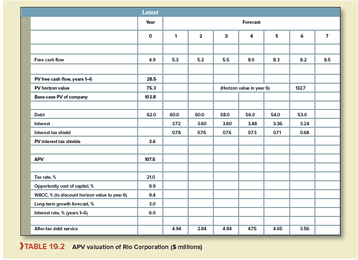
an increase of $1.0 million from NPV in Table 19.1. The increase can be traced to the higher early debt levels and to the assumption that the debt levels and interest tax shields are fixed and safe.[5]
Now a difference of $1.0 million is not a big deal, considering all the lurking risks and pitfalls in forecasting Rio’s free cash flows. But you can see the advantage of the flexibility that APV provides. The APV spreadsheet allows you to explore the implications of different financing strategies without locking into a fixed debt ratio or having to calculate a new WACC for every scenario.
APV is particularly useful when the debt for a project or business is tied to book value or has to be repaid on a fixed schedule. For example, Kaplan and Ruback used APV to analyze the prices paid for a sample of leveraged buyouts (LBOs). LBOs are takeovers, typically of mature companies, heavily debt-financed. However, the new debt is not intended to be permanent. LBO business plans call for generating extra cash by selling assets, shaving costs, and improving profit margins. The extra cash is used to pay down the LBO debt. Therefore, you can’t use WACC as a discount rate to evaluate an LBO because its debt ratio will not be constant.
APV works fine for LBOs. The company is first evaluated as if it were all-equity-financed. That means that cash flows are projected after tax, but without any interest tax shields generated by the LBO’s debt. The tax shields are then valued separately and added to the all-equity value. Any other financing side effects are added also. The result is an APV valuation for the company.[6] Kaplan and Ruback found that APV did a pretty good job explaining prices paid in these hotly contested takeovers, considering that not all the information available to bidders had percolated into the public domain. Kaplan and Ruback were restricted to publicly available data.
4. APV and Limits on Interest Deductions
The United States now limits the amount of interest that can be deducted for tax to 30% of each year’s EBITDA (or 30% of EBIT starting in 2022). Germany has a similar restriction, and the European Commission has proposed an EU-wide limit.
Most companies will not be caught by these rules. But what about the few that are caught? How should a financial manager take limits on interest-expense deductions into account?
Suppose the 30% constraint is and will be binding. Assume the firm is profitable and paying taxes. Then the future interest tax shields generated by a new investment project are proportional to its future EBITDA. The financial manager should forecast EBITDA and the associated tax shields and discount at a rate depending on the risk of EBITDA.[7] The APV formula is the same as before:
APV = base-case NPV + PV(interest tax shields)
but PV(interest tax shields) now depends on the project’s forecasted EBITDA.
Those projects that generate plenty of EBITDA will be especially valuable to tax-paying firms that are subject to the 30% constraint. The EBITDA of the project can relax the constraint for the firm as a whole, thus unlocking interest tax shields on the firm’s existing debt.
The APV of an entire business or company subject to the 30% constraint should also include the PV of interest tax shields generated by its expected future EBITDA. If the 30% limit on interest deductions is temporary—in one or two low-profit years, for example—then the unused tax shields are not lost but can be carried forward indefinitely and may therefore be merely delayed. The financial manager could assign the tax shields to future years, discount to PV and include them in APV.
5. APV for International Investments
APV is most useful when financing side effects are numerous and important. This is frequently the case for large international investments, which may have custom-tailored project financing and special contracts with suppliers, customers, and governments. Here are a few examples of financing side effects resulting from the financing of a project.
We explain project finance in Chapter 24. It typically means very high debt ratios to start, with most or all of a project’s early cash flows committed to debt service. Equity investors have to wait. Since the debt ratio will not be constant, you have to turn to APV.
Project financing may include debt available at favorable interest rates. Most governments subsidize exports by making special financing packages available, and manufacturers of industrial equipment may stand ready to lend money to help close a sale. Suppose, for example, that your project requires construction of an on-site electricity generating plant. You solicit bids from suppliers in various countries. Don’t be surprised if the competing suppliers sweeten their bids with offers of low interest rate project loans or if they offer to lease the plant on favorable terms. You should then calculate the NPVs of these loans or leases and include them in your project analysis.
Sometimes international projects are supported by contracts with suppliers or customers. Suppose a manufacturer wants to line up a reliable supply of a crucial raw material—powdered magnoosium, say. The manufacturer could subsidize a new magnoosium smelter by agreeing to buy 75% of production and guaranteeing a minimum purchase price. The guarantee is clearly a valuable addition to the smelter’s APV: If the world price of powdered magnoosium falls below the minimum, the project doesn’t suffer. You would calculate the value of this guarantee (by the methods explained in Chapters 20 to 22) and add it to APV.
Sometimes local governments impose costs or restrictions on investment or disinvestment. For example, Chile, in an attempt to slow down a flood of short-term capital inflows in the 1990s, required investors to “park” part of their incoming money in non-i nterest-bearing accounts for a period of two years. An investor in Chile during this period could have calculated the cost of this requirement and subtracted it from APV.30
I’ve been absent for some time, but now I remember why I used to love this website. Thank you, I will try and check back more frequently. How frequently you update your site?